Big-O in Practice: Choosing Data Structures That Keep Code Fast

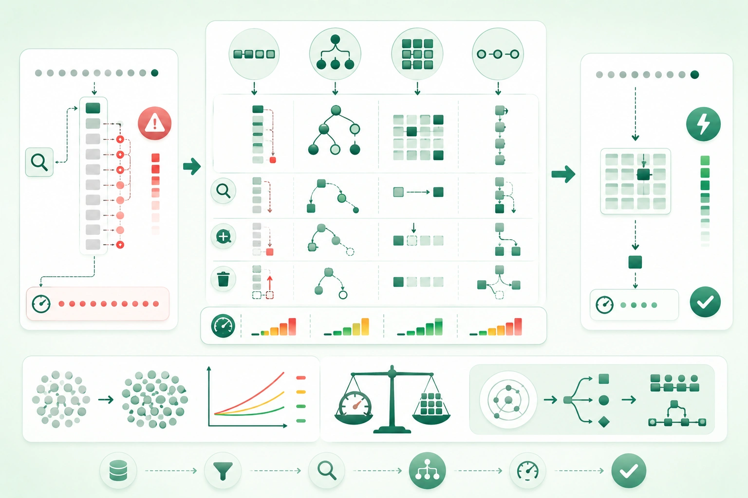
Big-O becomes useful when you stop treating it as:

a table to memorize

and start using it to answer:

What operation does this code
perform again and again?

How does that operation get more
expensive as the data grows?

A data structure is good when its cheap operations match your workload.

If your application repeatedly asks:

Does this ID exist?

then storing IDs in a list and scanning the entire list each time is usually a poor fit.

If your application repeatedly asks:

What is item number 250?

an indexed array-like structure is usually much more natural.

1. Read Big-O as a growth model

Big-O notation describes how work grows as input size:

n

becomes larger.

O(1)

Constant growth.

array[index]

is commonly treated as constant-time indexed access.

O(log n)

Logarithmic growth.

Each step removes a significant fraction of remaining possibilities.

Example:

binary search
in sorted array

O(n)

Linear growth.

scan every element once

O(n log n)

Common efficient comparison-sorting territory.

sort n items

O(n^2)

Quadratic growth.

compare every item
with every other item

Ignore constant multipliers for growth analysis

Big-O simplifies:

3n + 20

to:

O(n)

because the linear term dominates growth.

But constants still matter in real software

Two O(n) implementations can have very different:

CPU cost
memory allocation
cache behavior
network calls

Big-O tells you scaling shape, not exact milliseconds.

2. Find the operation your code performs most

Common data-structure operation costs (diagram)

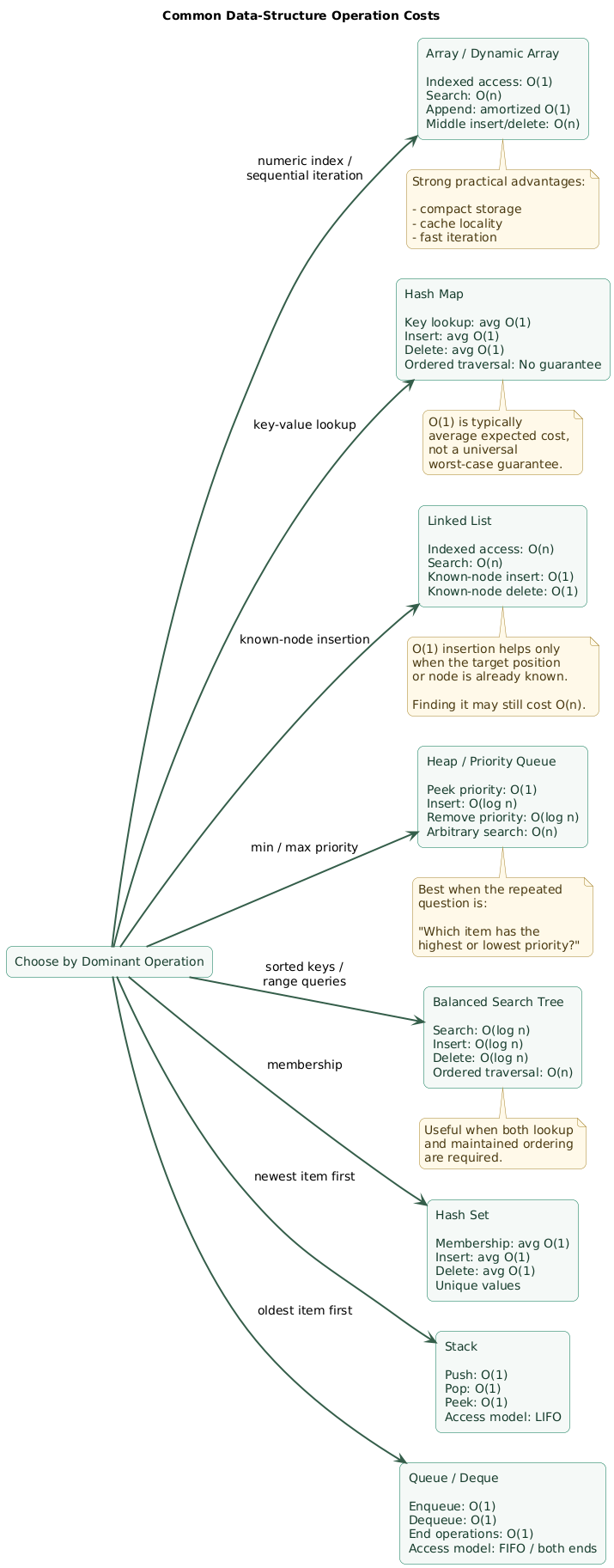
Before choosing a structure, list the operations.

Example: active sessions

Requirements:

add session

remove session

check whether session ID exists

occasionally iterate all sessions

The dominant operation may be:

membership lookup by ID

which strongly suggests a:

hash map
or
hash set

Example: timeline

Requirements:

append events

iterate in order

access by position

A dynamic array may be a natural fit.

Example: job scheduler

Requirement:

repeatedly retrieve
highest-priority job

A priority queue backed by a heap may fit better than sorting the complete list after every insertion.

Write the workload first

operation        frequency

lookup by ID     extremely high
append           high
delete           medium
ordered scan     rare

Then choose the representation.

3. Use arrays when indexing and iteration dominate

Arrays and dynamic arrays are excellent general-purpose structures.

Typical strengths

indexed access:
O(1)

iteration:
O(n)

append:
often amortized O(1)

Typical weakness

Inserting at the beginning:

[A B C D]

insert X at index 0

[X A B C D]

requires shifting existing elements in ordinary contiguous implementations.

That makes the operation:

O(n)

Removing from the middle also shifts elements

[A B C D E]

remove C

[A B D E]

elements after the removed position normally move.

Arrays often have excellent cache locality

Elements stored close together in memory can be efficient for:

iteration
sorting
numerical processing

Binary search changes lookup if the array is sorted

An arbitrary unsorted lookup is:

O(n)

but a sorted array can support binary search in:

O(log n)

while insertion may become expensive because order must be preserved.

Use arrays when

order matters
indexed access matters
iteration dominates
append is common

4. Use maps and sets for repeated lookup

Suppose you have:

100,000 blocked user IDs

and each incoming request asks:

is this user blocked?

List approach

for each request:
    scan blockedUsers

Membership check:

O(n)

Set approach

blockedUsers.contains(userId)

with a typical hash set:

average O(1)

This difference compounds

If:

m requests

each scan:

n blocked users

the naive workflow approaches:

O(mn)

while constructing a set once gives approximately:

O(n)
+
m average O(1) lookups

Use a map when values belong to keys

userId -> User

productCode -> Product

countryCode -> TaxRule

Use a set when only membership matters

seen IDs

permissions

blocked tokens

unique tags

Hashing has real costs

Hash structures trade extra memory and hashing work for fast expected lookup.

For a tiny collection:

5 items

a simple array scan can still be perfectly adequate.

5. Understand where linked lists actually help

Linked lists are often introduced as:

fast insertion
fast deletion

but this description leaves out the critical question:

Do you already know
which node to modify?

Finding an arbitrary value

head
 ↓
A -> B -> C -> D -> E

usually requires traversing:

O(n)

Insertion after a known node

If you already have a reference to:

C

linking:

C -> X -> D

can be constant-time.

But searching first changes the complete operation

find C:
O(n)

insert after C:
O(1)

total:
O(n)

Linked lists also have memory overhead

Nodes often store:

value
pointer to next
possibly pointer to previous

and nodes may be scattered across memory.

Do not choose a linked list from complexity tables alone

Arrays frequently perform extremely well in real programs because of contiguous storage, iteration speed, and lower overhead.

6. Use stacks, queues, and deques for access order

Stack

Last in, first out:

push
push
push

pop newest item

Useful for:

undo
DFS traversal
parser state
call-like workflows

Queue

First in, first out:

enqueue
enqueue
enqueue

dequeue oldest item

Useful for:

work processing
BFS traversal
message buffering
request scheduling

Deque

Efficient operations at both ends.

push front
push back
pop front
pop back

Avoid using the wrong end of an array accidentally

If your dynamic array has:

fast append

but

O(n) remove-from-front

then repeatedly implementing a queue as:

append at end
remove index 0

can create unnecessary repeated shifting.

Use a real queue or deque abstraction provided by the language or library.

7. Use heaps when priority matters

Consider:

100,000 pending jobs

and you repeatedly need:

job with smallest deadline

Scanning every time

find minimum:
O(n)

repeated many times becomes expensive.

Sorting after every insertion

may do more work than necessary.

Heap / priority queue

commonly provides:

inspect minimum:
O(1)

insert:
O(log n)

remove minimum:
O(log n)

for a min-heap style implementation.

Use when the repeated question is

what is the next highest-priority item?

Do not use a heap for arbitrary membership lookup

A heap is not a general:

find any item by ID quickly

structure.

You may combine:

heap
+
map

when a scheduler needs both:

priority selection
and
keyed lookup

8. Use ordered trees when order and range queries matter

Hash maps are excellent when you ask:

Give me exactly key K

but less useful when you ask:

Give me every key
between A and M

Balanced search tree

typically supports:

search:
O(log n)

insert:
O(log n)

delete:
O(log n)

while maintaining sorted order.

Useful for

ordered maps

ordered sets

range queries

predecessor / successor

sorted iteration

Hash map versus ordered tree

Need exact key lookup only?
Hash map often simpler.

Need ordered traversal?
Tree may fit.

Need range query?
Tree may fit.

Need min / max repeatedly?
Tree or heap depending on other operations.

Do not implement your own balanced tree casually

Use the standard library or a mature collection library where available.

9. Analyze the complete workflow, not one operation

Data-structure selection decision tree (diagram)

Complexity mistakes often happen because a developer optimizes:

one line

instead of:

the repeated workflow

Example: duplicate detection

Naive:

for each item:
    scan all previous items

can approach:

O(n^2)

Set-based approach

seen = set

for each item:
    if item in seen:
        duplicate
    else:
        add item

is typically:

O(n)

expected overall with ordinary hash-set assumptions.

Example: repeated search

Suppose:

n records

m lookup queries

scanning each time costs:

O(mn)

Building an index:

O(n)

followed by expected constant-time hash lookups can reduce repeated work substantially.

Precomputation can be worthwhile

Spending:

O(n)

once to construct:

map
set
index

is useful when the result supports many later operations.

But not always

If you need:

one lookup
in 10 items

a plain scan may remain simpler and fast enough.

10. Spot hidden repeated scans and nested work

Classic nested scan

for user in users:
    for order in orders:
        if order.userId == user.id:
            ...

If both collections grow with:

n

this approaches:

O(n^2)

Build an index instead

ordersByUser = map

for order in orders:
    ordersByUser[order.userId].append(order)

for user in users:
    userOrders = ordersByUser[user.id]

Construction and traversal can be much closer to:

O(users + orders)

Nested loops are not automatically quadratic

Example:

for chunk in chunks:
    for item in chunk:
        process(item)

If every item appears in exactly one chunk, total work may still be:

O(n)

Count total visits

Ask:

How many times can
one data element be processed?

Watch library calls inside loops

for item in items:
    if list.contains(item):
        ...

may hide:

O(n)
inside
O(n) loop

producing:

O(n^2)

11. Distinguish average, worst-case, and amortized cost

Average case

Describes expected behavior under an assumed distribution or normal implementation conditions.

Hash-table lookup is commonly described as:

average O(1)

Worst case

Describes the upper growth bound for difficult inputs or structure states.

Depending on implementation and collision behavior, hash-table operations can degrade beyond their average case.

Amortized analysis

Dynamic arrays often append in:

amortized O(1)

because most appends simply use available capacity.

Occasionally:

buffer full
      ↓
allocate larger buffer
      ↓
copy existing elements

causes:

O(n)

work for that individual append.

Across many appends, the average per operation remains constant under standard geometric growth strategies.

Know which complexity guarantee your library actually offers

Do not blindly transfer:

generic textbook claim

to:

specific runtime implementation

when performance is critical.

12. Include memory and cache locality in the decision

Big-O time complexity is only one dimension.

Array

Often compact:

value
value
value
value

with good spatial locality.

Hash map

May require:

buckets
hash metadata
unused capacity
key storage
value storage

Linked structure

Each node may require:

value
next pointer
previous pointer

plus allocator overhead.

Memory affects speed too

CPU caches make:

contiguous sequential access

particularly efficient.

This is one reason a theoretically attractive pointer-heavy structure can lose to an array in real workloads.

Space complexity matters at scale

A lookup table that saves CPU may consume:

additional O(n) memory

which can be worthwhile or unacceptable depending on:

device memory
server density
dataset size
latency target

13. Match complexity to realistic data size

Growth-rate practical impact (diagram)

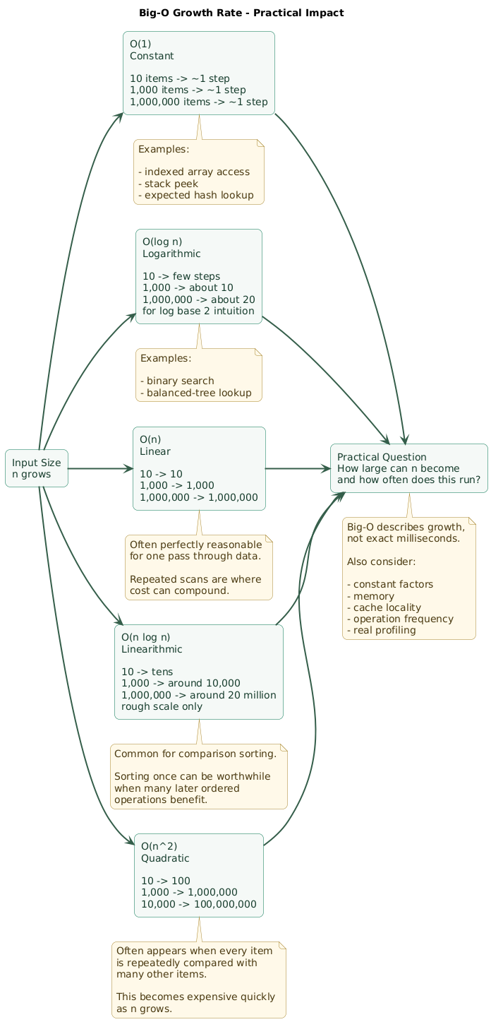
Suppose your list always contains:

8 menu items

An O(n) scan is unlikely to be a meaningful problem.

Small bounded collections change priorities

For:

n <= 10

clarity may matter much more than replacing:

linear scan

with a more complicated index.

Unbounded growth changes priorities

If:

n = number of users

and the system can grow from:

1,000
to
10,000,000

an O(n) operation on every request deserves more attention.

Quadratic growth becomes painful quickly

Roughly:

100 items:
10,000 pair checks

1,000 items:
1,000,000 pair checks

10,000 items:
100,000,000 pair checks

Ask for a realistic upper bound

How large is n today?

How large can n become?

How frequently does operation run?

Is it interactive or offline?

Is latency user-visible?

Frequency matters as much as collection size

An O(n) batch job once per night may be harmless.

The same scan executed:

50,000 times per second

is a different engineering problem.

14. Profile and benchmark after choosing sensibly

Big-O helps predict scaling risk.

Profiling tells you:

where your program
is actually slow

Use complexity during design

Avoid obvious traps such as:

repeated full scan
inside another full scan

when a map can eliminate repeated work.

Then profile the real application

Measure:

CPU time
allocations
memory
database calls
cache misses
latency
throughput

Benchmark representative inputs

Do not benchmark only:

n = 10

if production uses:

n = 1,000,000

Warm-up and runtime behavior can matter

Managed runtimes may include:

JIT compilation
garbage collection
runtime optimization

which can distort naive microbenchmarks.

Benchmark the complete operation

If replacing:

array

with:

hash map

include:

construction
lookup
updates
memory

rather than measuring only one lookup.

Do not optimize complexity nobody pays for

A readable O(n) solution for:

12 configuration entries

may be superior to a complex caching layer.

15. Copy/paste data-structure checklist

Big-O and data-structure checklist

Start with workload
- What is n?
- How large is n today?
- How large can n become?
- How frequently does this code run?
- Which operation dominates?
- Is the path user-facing?
- Is the workload latency-sensitive?
- Is it batch processing?

Big-O basics
- O(1) means constant growth.
- O(log n) grows slowly.
- O(n) grows linearly.
- O(n log n) is common for efficient comparison sorting.
- O(n^2) grows quickly.
- Ignore constants for asymptotic classification.
- Remember constants still matter in real runtime.

Arrays
- Use for indexed access.
- Use for ordered iteration.
- Use for append-heavy workloads.
- Indexed lookup is typically O(1).
- Linear search is O(n).
- Insertion near front is commonly O(n).
- Deletion from middle is commonly O(n).
- Sorting enables binary search.
- Arrays often have good cache locality.

Dynamic arrays
- Append is commonly amortized O(1).
- Occasional resize can be O(n).
- Reserve capacity when API supports it and size is predictable.
- Avoid repeated front removal for queue behavior.
- Measure allocation growth when extremely large.

Hash maps
- Use for key-value lookup.
- Expected lookup is commonly O(1).
- Expected insert is commonly O(1).
- Expected delete is commonly O(1).
- Requires hashing.
- Requires extra memory.
- Key equality must be correct.
- Hash quality matters.
- Do not assume sorted order.

Hash sets
- Use for membership tests.
- Use for duplicate detection.
- Use for deduplication.
- Use for intersection / difference style operations where appropriate.
- Expected membership is commonly O(1).
- Do not use list scan repeatedly when membership dominates.

Linked lists
- Finding arbitrary element is O(n).
- Insert after known node can be O(1).
- Delete known node can be O(1) depending on representation.
- Random indexed access is O(n).
- Nodes have pointer overhead.
- Cache locality may be poor.
- Do not choose only because insertion looks O(1) in a table.

Stacks
- Use LIFO semantics.
- Push should be cheap.
- Pop should be cheap.
- Useful for DFS.
- Useful for undo.
- Useful for parser state.
- Avoid arbitrary lookup expectations.

Queues
- Use FIFO semantics.
- Enqueue should be cheap.
- Dequeue should be cheap.
- Useful for BFS.
- Useful for job processing.
- Useful for buffering.
- Avoid array-front shifting if runtime structure makes it O(n).

Deques
- Use when both ends matter.
- Push front.
- Push back.
- Pop front.
- Pop back.
- Useful for sliding-window algorithms.
- Useful for queue + stack hybrid access.

Heaps
- Use when priority dominates.
- Peek min / max is typically O(1).
- Insert is typically O(log n).
- Remove priority element is typically O(log n).
- Arbitrary search is not the main strength.
- Use priority queue abstraction when available.

Balanced trees
- Search is typically O(log n).
- Insert is typically O(log n).
- Delete is typically O(log n).
- Preserve ordering.
- Useful for range queries.
- Useful for predecessor / successor.
- Useful for ordered maps and sets.

Sorting
- Ask whether sorting once enables many later operations.
- Comparison sort is commonly O(n log n).
- Avoid sorting repeatedly when order has not changed.
- Consider maintaining ordered structure when updates and ordered queries mix.
- Use standard-library sort unless special requirements exist.

Binary search
- Requires sorted data.
- Search is O(log n).
- Maintaining sorted array can make insertion O(n).
- Good for mostly-static data with frequent lookups.
- Test boundaries carefully.

Linear scan
- Often simplest.
- O(n).
- Fine for small bounded collections.
- Fine for one-time passes.
- Avoid repeating scan unnecessarily.
- Prefer clarity when n is tiny.

Membership
- One membership test in small list may be fine.
- Many membership tests suggest set.
- Build set once when reused.
- Count construction cost.
- Count memory cost.

Duplicate detection
- Nested comparisons can be O(n^2).
- Hash set can often reduce expected workflow to O(n).
- Sorting can also support duplicate detection in O(n log n).
- Choose based on ordering and memory requirements.

Repeated lookup
- Avoid scanning same list repeatedly.
- Build index.
- Use map.
- Use set.
- Cache only when lifecycle and invalidation are clear.
- Include index-construction cost.

Nested loops
- Do not automatically label every nested loop O(n^2).
- Analyze actual loop bounds.
- Count how often each element is visited.
- Look for repeated scans.
- Look for hidden contains / find calls.
- Look for database calls inside loops.

N+1 patterns
- Complexity can include external operations.
- One query per item can dominate CPU complexity.
- Batch requests where appropriate.
- Preload related records.
- Measure network and database latency.

Average case
- Know whether complexity claim is average.
- Hash tables commonly use expected average behavior.
- Input distribution matters.
- Implementation details matter.

Worst case
- Know whether adversarial input matters.
- Consider worst-case latency for security-sensitive paths.
- Consider real-time constraints.
- Read standard-library guarantees when critical.

Amortized complexity
- Understand dynamic-array growth.
- Understand occasional expensive operations.
- Evaluate cost across a sequence of operations.
- Do not confuse amortized O(1) with every operation taking constant time.

Memory
- Measure extra indexes.
- Measure hash-table capacity.
- Measure node overhead.
- Measure duplicated keys.
- Consider mobile / embedded memory constraints.
- Consider server density.

Cache locality
- Contiguous arrays often iterate efficiently.
- Pointer-heavy structures can cause cache misses.
- Big-O does not model locality.
- Benchmark hot loops.

Ordering
- Need original insertion order?
- Need sorted order?
- Need no order?
- Need range queries?
- Do not pay for order if unused.
- Do not lose order if contract requires it.

Duplicates
- Are duplicates allowed?
- Need uniqueness?
- Set may encode uniqueness directly.
- Multiset / counter may fit frequency counting.
- Map from value to count can support frequencies.

Index access
- Need item by numeric position?
- Array-like structure is natural.
- Linked list is usually poor for random access.
- Tree can support order statistics only with specialized augmentation.

Key lookup
- Need item by ID?
- Map usually fits.
- Avoid list scan on every request.
- Validate key equality and hashing.

Priority
- Need min or max repeatedly?
- Heap may fit.
- Need arbitrary ordered traversal too?
- Tree may fit better.
- Need both key lookup and priority?
- Consider combining structures carefully.

Ranges
- Need keys between low and high?
- Ordered tree may fit.
- Sorted array may fit for mostly-static data.
- Hash map does not naturally support range queries.

Top K
- Sorting everything can cost O(n log n).
- Heap can help when k is much smaller than n.
- Measure whether full sort is already cheap enough.
- Use library algorithms when available.

Queues at scale
- Use queue abstraction.
- Avoid shifting entire array repeatedly.
- Consider bounded queue.
- Consider backpressure.
- Consider concurrent queue requirements separately.

Graphs
- Adjacency list is often efficient for sparse graphs.
- Adjacency matrix uses O(V^2) memory.
- Matrix can provide constant-time edge existence.
- Choose based on density and operations.

Strings
- Understand string concatenation complexity in your runtime.
- Avoid repeated copying in loops when builder exists.
- Remember Unicode length semantics are separate from Big-O.
- Benchmark large text transformations.

Immutability
- Persistent data structures may trade write cost and memory for safer sharing.
- Copy-on-write behavior can change practical cost.
- Understand runtime semantics.

Copying
- Slicing may copy or reference depending on runtime.
- Passing collections may copy or share depending on language.
- Hidden O(n) copies can dominate loops.
- Review serialization boundaries.

Recursion
- Time complexity and stack complexity are separate.
- Deep recursion can overflow stack.
- Tail-call behavior differs by runtime.
- Iterative structure may be safer for deep data.

Space complexity
- Track extra O(n) indexes.
- Track recursion stack.
- Track temporary arrays.
- Track caches.
- Track duplicate representations.
- Balance speed against memory.

Small data
- Prefer simple code.
- O(n) may be completely adequate.
- Avoid elaborate indexing for five elements.
- Keep optimization proportional to scale.

Large data
- Avoid repeated full scans.
- Avoid quadratic workflows.
- Build indexes.
- Stream when full materialization is unnecessary.
- Batch external operations.
- Consider memory limits.

Real-time paths
- Prefer predictable latency.
- Consider worst-case behavior.
- Avoid unexpected resizing if strict latency matters.
- Preallocate where appropriate.
- Avoid garbage-heavy structures when latency-sensitive.

Batch paths
- Higher one-time setup cost may be acceptable.
- Sorting once may simplify workflow.
- Building index may pay off.
- Parallelism is separate from algorithmic complexity.

Profiling
- Profile before complex optimization.
- Find actual hot path.
- Measure CPU.
- Measure allocations.
- Measure I/O.
- Measure database queries.
- Measure latency distribution.

Benchmarking
- Use representative data sizes.
- Include warm-up where runtime requires it.
- Repeat measurements.
- Avoid benchmarking debug builds.
- Avoid unrealistic microbenchmarks.
- Compare complete workflow.

Optimization
- Fix algorithmic problems before micro-optimizing instructions.
- Replace O(n^2) workflow before shaving nanoseconds from O(1).
- Keep readability.
- Measure after change.
- Verify memory impact.

Code review
- What is n?
- Which operation dominates?
- Does lookup scan a list repeatedly?
- Is contains hidden inside a loop?
- Is sorting repeated unnecessarily?
- Is data structure preserving unused order?
- Is extra index worth the memory?
- Is complexity average or guaranteed?
- Is input bounded?
- Has real performance been measured?

Final review
- Is the dominant operation identified?
- Does the chosen structure make that operation cheap?
- Is indexed access required?
- Is keyed lookup required?
- Is membership required?
- Is sorted order required?
- Are range queries required?
- Is FIFO or LIFO behavior required?
- Is priority retrieval required?
- Are duplicate rules explicit?
- Is the complete workflow analyzed rather than one line?
- Are repeated scans eliminated where they matter?
- Are average, worst-case, and amortized costs understood?
- Is memory overhead acceptable?
- Is cache locality relevant?
- Is realistic maximum n known?
- Is operation frequency known?
- Is the simple solution fast enough?
- Has the real workload been profiled?
- Is the final code still understandable?

16. FAQ

What does Big-O notation mean?

Big-O describes how resource use grows as input size grows. It is most useful for comparing scaling behavior rather than predicting exact execution time.

Is O(1) always faster than O(n)?

No. A small O(n) loop can be faster than an O(1) operation with large constant overhead. Big-O becomes increasingly useful as input size grows and when an operation is repeated frequently.

When should I replace a list with a set?

When repeated membership checks dominate and ordering or duplicate preservation is not the main requirement. A set can often replace repeated O(n) scans with expected constant-time membership checks.

Why is append to a dynamic array amortized O(1)?

Most appends use already allocated capacity and are constant-time. Occasionally the structure allocates a larger buffer and copies existing values. Across many appends, that expensive resize is spread across many cheap operations.

Are linked lists faster than arrays for insertion?

Only in the right circumstances. Inserting after a node you already have can be constant-time, but finding that node may require O(n) traversal. Arrays also tend to benefit from better memory locality.

When should I use a heap?

Use a heap-backed priority queue when you repeatedly need the smallest or largest priority item while also inserting new items efficiently.

Should I always optimize the best Big-O complexity?

No. Choose a sensible structure based on expected growth and workload, then profile the real system. Small bounded collections often favor simple code even when a theoretically faster structure exists.

Key terms (quick glossary)

Big-O notation

A notation describing an upper growth rate for resource usage as input size increases.

Time complexity

A model of how the amount of computational work grows relative to input size.

Space complexity

A model of how additional memory usage grows relative to input size.

O(1)

Constant growth, where the modeled amount of work does not increase with input size.

O(log n)

Logarithmic growth, commonly seen when each operation substantially reduces the remaining search space.

O(n)

Linear growth, commonly produced by processing every input element once.

O(n log n)

A growth rate commonly associated with efficient comparison-based sorting algorithms.

O(n^2)

Quadratic growth, often caused by comparing or combining many pairs of elements.

Amortized complexity

The average cost per operation across a sequence in which occasional operations are substantially more expensive than ordinary ones.

Hash map

A key-value data structure that uses hashing to provide fast expected lookup, insertion, and deletion.

Hash set

A hashing-based collection representing unique values and supporting fast expected membership tests.

Heap

A partially ordered tree-like structure commonly used to implement priority queues.

Balanced search tree

An ordered tree that maintains bounded height so search, insertion, and deletion remain logarithmic.

Cache locality

The performance advantage obtained when data accessed close together in time is also stored close together in memory.

Dominant operation

The operation or set of operations whose frequency and cost have the greatest effect on a workload.

Worst-case complexity

The growth of resource usage for the most expensive valid input or internal state covered by the analysis.