Time Series Backtesting Basics: Seasonality, Drift, and Realistic Evaluation

Forecasting models have a special evaluation problem: the future is not interchangeable with the past.

A random train-test split can quietly let a model learn from observations that occurred after the periods it is asked to predict. Even when there is no obvious target leakage, neighboring observations can share trend, seasonal context, promotions, weather, inventory conditions, or other time-dependent information.

A realistic backtest instead simulates a sequence of historical production forecasts. At each simulated prediction date, the model should receive only the information that would have existed then.

1. Why random train-test splits fail for forecasting

Ordinary random cross-validation assumes that exchanging observations between train and validation sets does not fundamentally change the prediction problem.

Time series usually violates that assumption.

Bad evaluation direction

January 2026  → validation
February 2026 → training
March 2026    → training
April 2026    → validation

A real February model cannot use March observations to predict January.

Correct forecasting direction

past observations
      ↓
fit model
      ↓
future observations

This is why time-aware cross-validation keeps training observations before validation observations.

Chronological holdout

The simplest valid design is often one historical/future split:

train = df[df["date"] < "2026-01-01"]

test = df[df["date"] >= "2026-01-01"]

That is much better than random splitting, but one test period can still provide an unstable estimate when seasonality or business conditions vary.

Rolling backtests solve this by simulating several historical forecast origins.

2. Rolling-origin backtesting

Rolling-origin backtesting workflow (diagram)

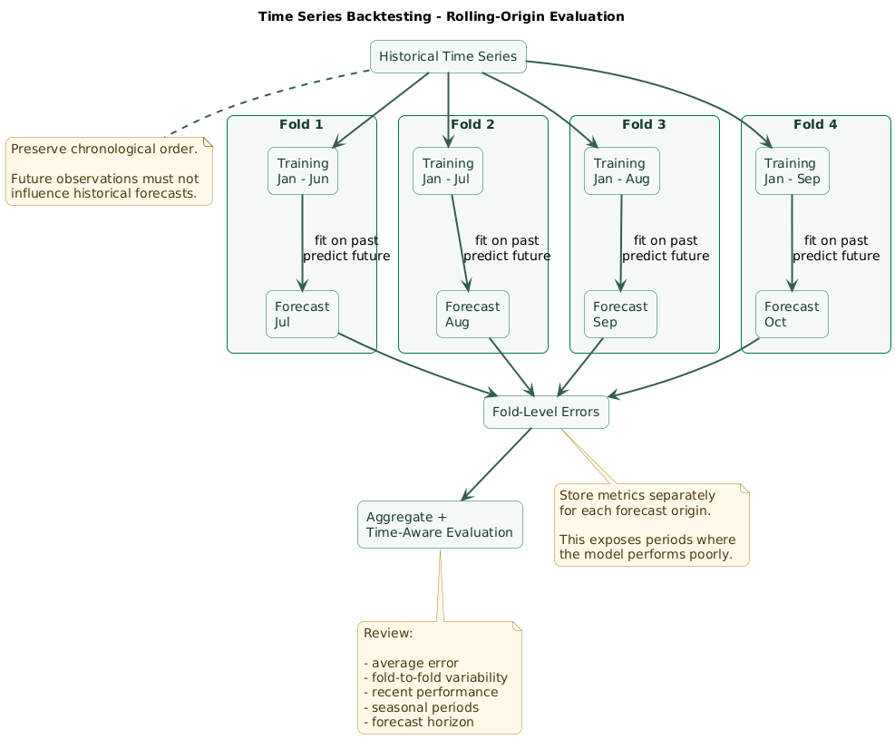
Rolling-origin evaluation is also called walk-forward validation.

Instead of evaluating once, move the simulated prediction date through history:

Fold 1:
Train: Jan - Jun
Test:  Jul

Fold 2:
Train: Jan - Jul
Test:  Aug

Fold 3:
Train: Jan - Aug
Test:  Sep

Fold 4:
Train: Jan - Sep
Test:  Oct

Each fold answers:

If the model had been trained at this historical point, how well would it have predicted what happened next?

TimeSeriesSplit

from sklearn.model_selection import TimeSeriesSplit

cv = TimeSeriesSplit(
    n_splits=5
)

for fold, (train_idx, test_idx) in enumerate(
    cv.split(X),
    start=1
):
    X_train = X.iloc[train_idx]
    X_test = X.iloc[test_idx]

    y_train = y.iloc[train_idx]
    y_test = y.iloc[test_idx]

    print(
        fold,
        X_train.index.min(),
        X_train.index.max(),
        X_test.index.min(),
        X_test.index.max()
    )

Scikit-learn's TimeSeriesSplit creates successive training sets that contain earlier observations and later test sets. Its test_size, max_train_size, and gap arguments allow further control over the historical simulation.

Equal time duration matters

If you want errors from different folds to represent comparable calendar horizons, observations should correspond to a consistent time spacing or you should build the folds explicitly from timestamps.

One hundred rows can represent 100 days in one fold and six months in another when event frequency is irregular.

3. Expanding vs sliding training windows

Expanding window

An expanding window retains every historical observation available at the forecast origin.

Fold 1:
[train train train] [test]

Fold 2:
[train train train train] [test]

Fold 3:
[train train train train train] [test]

This is a strong default when older data remains relevant and more history improves estimation.

Sliding window

A sliding window keeps only a fixed amount of recent history.

Fold 1:
[train train train] [test]

Fold 2:
      [train train train] [test]

Fold 3:
            [train train train] [test]

This can help when the data-generating process changes and observations from several years ago describe a regime that no longer exists.

Limit training history with max_train_size

cv = TimeSeriesSplit(
    n_splits=5,
    test_size=30,
    max_train_size=365
)

For daily observations, this configuration can approximate training on the most recent 365 samples and evaluating on 30 later samples per fold, assuming each sample represents the intended regular time unit.

Do not assume more history is always better

Old data adds sample size but can also add obsolete relationships.

Compare:

• All available history.
• Last 24 months.
• Last 12 months.
• Last relevant seasonal cycles.

Use the same backtest periods so window length is the variable being tested.

4. Match the forecast horizon to production

A one-day-ahead model and a 30-day-ahead model solve different problems.

Do not evaluate one horizon and deploy another.

Example production requirement

Every Monday:
forecast demand for the next 7 days.

The backtest should therefore contain historical Monday forecast origins with seven-day forecast windows.

Multi-step error usually changes with horizon

Measure errors separately for:

horizon 1
horizon 2
horizon 3
...
horizon 7

An average across all seven steps can hide severe deterioration at the longest horizon.

results.groupby(
    "forecast_horizon"
)["absolute_error"].mean()

Use a gap when information has a delay

Suppose the newest seven days of target data are not finalized when the forecast is produced.

Training directly up to the forecast origin would use data unavailable in production.

cv = TimeSeriesSplit(
    n_splits=5,
    test_size=14,
    gap=7
)

A gap can also help when features near the prediction boundary contain information that overlaps with the forecast window.

5. Prevent future-data leakage in features

Correct chronological folds do not protect you if feature engineering already used future values.

Lag features

df["lag_1"] = (
    df["sales"].shift(1)
)

df["lag_7"] = (
    df["sales"].shift(7)
)

These use values observed before the current target.

Rolling mean: shift before rolling when necessary

df["previous_7d_mean"] = (
    df["sales"]
      .shift(1)
      .rolling(7)
      .mean()
)

Without the shift, the current target can enter its own predictor.

Centered rolling windows are dangerous

# Usually inappropriate for forecasting features
df["centered_mean"] = (
    df["sales"]
      .rolling(
          window=7,
          center=True
      )
      .mean()
)

A centered window includes later observations around each timestamp.

External regressors must be available in the future

Imagine forecasting sales seven days ahead using:

• Weather.
• Price.
• Promotion schedule.
• Inventory.

Ask whether production knows the future value.

A planned promotion may be known. The actual temperature seven days later is not. You may have a weather forecast, but that is different from using the realized future weather observed in historical data.

Historical feature generation should be point-in-time correct

For every backtest origin, reconstruct features from information available at that origin.

6. Make seasonality part of the backtest

Seasonality, drift, and backtest diagnostics (diagram)

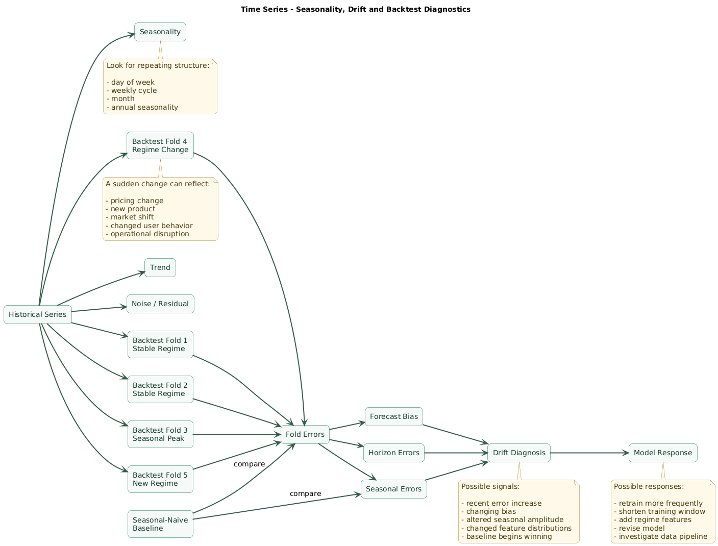
Seasonality means patterns repeat at a meaningful period.

Examples include:

• Hourly patterns within a day.
• Weekday vs weekend behavior.
• Weekly cycles.
• Monthly billing patterns.
• Annual holidays and weather seasons.

Backtests must cover the cycles you expect in production

Evaluating only January and February may tell you little about a model deployed through summer and the holiday season.

Report error by meaningful calendar period:

results["month"] = (
    results["timestamp"].dt.month
)

mae_by_month = (
    results.groupby("month")
           .apply(
               lambda g:
               (g["actual"] - g["forecast"])
               .abs()
               .mean()
           )
)

Inspect seasonal structure

Decomposition can help reveal whether the series contains trend, seasonality, and residual behavior.

from statsmodels.tsa.seasonal import STL

result = STL(
    series,
    period=7,
    robust=True
).fit()

trend = result.trend
seasonal = result.seasonal
residual = result.resid

Here, a period of seven would represent a seven-observation cycle when that is meaningful for the series.

Decomposition is a diagnostic tool, not permission to use future seasonal components when building historical prediction features. Keep the point-in-time boundary intact.

Multiple seasonalities

Hourly data may exhibit both daily and weekly patterns. Sales can show weekly and annual seasonality simultaneously.

Your backtest should span enough time for important cycles to appear and should include baseline features or models capable of representing them.

7. Beat naive and seasonal-naive baselines

Forecasting models should beat simple forecasts that exploit the obvious time structure.

Persistence baseline

forecast[t] = actual[t - 1]

In pandas:

df["naive_forecast"] = (
    df["target"].shift(1)
)

Seasonal-naive baseline

If a daily series has strong weekly seasonality:

df["seasonal_naive"] = (
    df["target"].shift(7)
)

For monthly data with an annual cycle:

df["seasonal_naive"] = (
    df["target"].shift(12)
)

Why simple baselines matter

A gradient-boosting model may appear accurate in absolute terms but offer almost no improvement over “same day last week.”

Complexity is justified by incremental value:

MAE seasonal naive:  12.4
MAE model:           12.1

That 0.3 improvement should be judged against engineering complexity, inference cost, retraining requirements, and business value.

Baseline performance can change with drift

Seasonal persistence may dominate in stable periods and fail suddenly after a pricing change, new product launch, economic shock, or altered customer behavior.

Compare baselines in every backtest fold, not only globally.

8. Choose forecast metrics carefully

Mean Absolute Error

from sklearn.metrics import mean_absolute_error

mae = mean_absolute_error(
    y_true,
    y_pred
)

MAE measures the average absolute error in the same units as the target.

This makes statements such as “the forecast misses by 14 orders on average” easy to interpret.

Root Mean Squared Error

from sklearn.metrics import (
    root_mean_squared_error
)

rmse = root_mean_squared_error(
    y_true,
    y_pred
)

RMSE penalizes large residuals more strongly than MAE, which can be useful when large misses are disproportionately costly.

MAPE

from sklearn.metrics import (
    mean_absolute_percentage_error
)

mape = mean_absolute_percentage_error(
    y_true,
    y_pred
)

Percentage errors are easy to communicate, but MAPE becomes problematic when actual values are zero or very close to zero because the denominator can make the metric extremely large.

Before using percentage error, inspect the target distribution and decide whether percentage interpretation is meaningful.

Do not average away the important structure

Report error by:

• Forecast horizon.
• Backtest fold.
• Month or season.
• Weekday.
• Product or location.
• Demand volume.

fold_metrics = (
    predictions
      .groupby("fold")
      .apply(
          lambda x: mean_absolute_error(
              x["actual"],
              x["forecast"]
          )
      )
)

print(fold_metrics)

Inspect forecast bias

predictions["error"] = (
    predictions["forecast"]
    - predictions["actual"]
)

mean_error = (
    predictions["error"].mean()
)

An average signed error above zero suggests systematic overforecasting; below zero suggests underforecasting.

A model can have acceptable MAE while maintaining a directional bias that causes inventory or staffing problems.

9. Detect drift and regime changes

Time-series data can change because the world generating it changes.

Possible drift signals

• The target level moves permanently.
• Variance increases.
• Seasonal amplitude changes.
• A weekly pattern disappears.
• Feature distributions shift.
• The relationship between features and the target changes.
• Forecast error increases in recent folds.

Track backtest error chronologically

fold_results = pd.DataFrame({
    "fold_end": fold_end_dates,
    "mae": fold_mae
}).sort_values("fold_end")

print(fold_results)

Imagine:

2025 Q1: MAE 10.2
2025 Q2: MAE 10.7
2025 Q3: MAE 11.0
2025 Q4: MAE 10.5
2026 Q1: MAE 18.9
2026 Q2: MAE 21.3

The overall historical average hides a major recent deterioration.

Compare expanding and recent-window models

If drift is present, train two versions:

Model A:
all historical observations

Model B:
most recent 12 months

A recent-window model may sacrifice sample size but adapt better to the current regime.

Do not automatically delete history

Old data may still contain valuable seasonal events that recent windows do not contain.

For example, a twelve-month training window contains only one example of each annual holiday period.

Backtesting should determine whether recency or longer seasonal history is more valuable.

Regime features can sometimes help

Known structural changes can be represented explicitly:

• Price-policy change.
• Store opening.
• Product redesign.
• New market launch.
• Changed subscription model.

But the feature must represent information actually known when the forecast is made.

10. Turn backtesting into a production evaluation plan

Time-series backtest trust checklist (diagram)

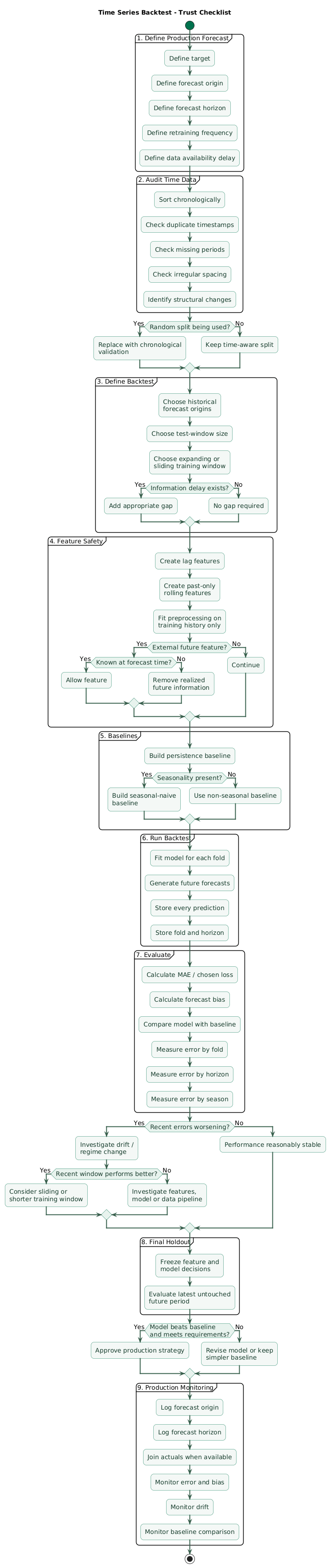
Match retraining behavior

If production retrains every Monday, a realistic backtest can simulate weekly retraining rather than fitting a new model after every individual observation.

If production retrains monthly, evaluate monthly origins.

Separate model selection from the final period

Repeated rolling folds can be used for:

• Feature design.
• Model selection.
• Hyperparameter selection.
• Training-window selection.

Preserve a final later period that does not influence those decisions.

Development:
2022-01 through 2025-12

Final holdout:
2026-01 through 2026-06

After the approach is chosen using historical backtests, evaluate the frozen strategy on the final holdout.

Evaluate the complete pipeline

Every backtest fold should recreate:

1. Historical feature construction.
2. Imputation.
3. Scaling or encoding where relevant.
4. Model fitting.
5. Forecast generation.
6. Post-processing.

Do not preprocess the entire series first when that preprocessing learns information from later observations.

Store fold-level predictions

Saving only one MAE number throws away diagnostic information.

prediction_log = pd.DataFrame({
    "timestamp": timestamps,
    "fold": fold_ids,
    "horizon": horizons,
    "actual": actual,
    "forecast": forecast
})

prediction_log["error"] = (
    prediction_log["forecast"]
    - prediction_log["actual"]
)

This lets you later inspect:

• Which dates were difficult.
• Which horizons failed.
• Whether errors became biased.
• Whether holidays caused failures.
• Whether drift appeared after a specific date.

Production monitoring should resemble backtest reporting

Monitor:

• Forecast error once actuals arrive.
• Error by forecast horizon.
• Bias.
• Target distribution.
• Feature distribution.
• Missing feature rates.
• Seasonal performance.
• Model-vs-baseline improvement.

If a seasonal-naive baseline starts beating the production model, that is useful evidence that retraining, model redesign, or feature investigation is needed.

11. Copy/paste time-series backtesting checklist

Time-series backtesting checklist

Production definition
- Define exactly what is being forecast.
- Define the forecast origin.
- Define the forecast horizon.
- Define forecast frequency.
- Define model retraining frequency.
- Define when target values become finalized.
- Define which external variables are known at forecast time.
- Define operational costs of overforecasting and underforecasting.

Raw time series
- Parse timestamps explicitly.
- Sort observations chronologically.
- Check duplicate timestamps.
- Check missing timestamps.
- Check irregular spacing.
- Confirm timezone assumptions.
- Identify frequency changes.
- Identify missing target periods.
- Identify historical data corrections.
- Record structural business changes.

Validation design
- Do not use ordinary random train-test splitting for forecasting.
- Keep training observations earlier than validation observations.
- Choose realistic historical forecast origins.
- Match test-window length to the production horizon.
- Use actual timestamps when row spacing is irregular.
- Cover enough backtest origins to assess stability.
- Preserve a final later holdout when possible.

Rolling-origin evaluation
- Define the first training period.
- Define test-window size.
- Define how far the origin moves between folds.
- Decide whether each fold retrains the model.
- Record train start and train end for every fold.
- Record test start and test end for every fold.
- Save every fold's predictions.
- Save every fold's metrics.

Expanding windows
- Use expanding history when old observations remain informative.
- Confirm training size grows as expected.
- Consider computational cost as history expands.
- Compare expanding performance with recent-window alternatives.

Sliding windows
- Consider sliding windows when drift makes old data less relevant.
- Choose window length using historical backtests.
- Retain enough periods to represent important seasonality.
- Do not shorten the window only because recent folds look better.
- Compare the same evaluation periods across window strategies.

Forecast horizon
- Match the evaluated horizon to production.
- Evaluate each forecast step separately.
- Check whether error grows with horizon.
- Avoid evaluating one-step forecasts when production requires multi-step forecasts.
- Reproduce recursive or direct forecasting behavior used in deployment.
- Record the horizon with each prediction.

Gap
- Check whether recent targets are finalized at forecast time.
- Add a gap when labels arrive with delay.
- Add a gap when overlapping windows create contamination.
- Match the gap to real information latency.
- Do not use observations that production would not yet know.

Lag features
- Shift target values before using them as predictors.
- Verify lag 1 really means one production time unit.
- Add seasonal lags where meaningful.
- Check missing values created by lagging.
- Prevent the target from entering its own predictors.

Rolling features
- Use past-only rolling windows.
- Shift before rolling when the current value must be excluded.
- Avoid centered rolling windows for historical forecast features.
- Calculate rolling aggregates separately at the correct point-in-time boundary.
- Check minimum history requirements.
- Prevent future rows from entering aggregates.

External variables
- Distinguish known future values from realized future values.
- Use scheduled promotions only if the schedule was available.
- Do not use realized future weather when production only has a forecast.
- Do not use corrected future inventory states.
- Version external data when historical availability matters.

Preprocessing
- Fit learned transformations within each training fold.
- Fit scalers on historical training data only.
- Fit imputers on training data only.
- Fit encoders on training data only.
- Fit dimensionality reduction on training data only.
- Apply fitted transformations to the future validation period.
- Use Pipeline where appropriate.

Seasonality
- Identify plausible seasonal periods.
- Inspect day-of-week patterns.
- Inspect weekly patterns.
- Inspect monthly patterns.
- Inspect annual cycles.
- Cover important seasons in backtest folds.
- Compare error by season.
- Compare error around holidays.
- Consider STL or other decomposition for diagnostics.
- Avoid using future decomposition information in historical features.

Baselines
- Build a last-observation baseline.
- Build a seasonal-naive baseline when seasonality exists.
- Compare every model against the same baseline periods.
- Measure model improvement over baseline by fold.
- Investigate periods where the baseline wins.
- Do not justify complexity without meaningful incremental value.

Metrics
- Choose a metric aligned with operational cost.
- Report MAE when target-unit interpretation is useful.
- Consider RMSE when large errors deserve greater penalty.
- Use MAPE cautiously when actual values approach zero.
- Report signed forecast bias.
- Report error by horizon.
- Report error by fold.
- Report error by season.
- Report error by important segment.
- Avoid relying on one global average.

Drift
- Plot fold metrics chronologically.
- Compare recent error with older error.
- Monitor changes in target level.
- Monitor changes in variance.
- Monitor seasonal amplitude.
- Monitor feature distributions.
- Monitor forecast bias.
- Identify known regime changes.
- Compare long-history models with recent-window models.
- Document when relationships appear to change.

Hyperparameter tuning
- Tune using chronological backtest folds.
- Do not select parameters using the final future holdout.
- Keep feature engineering inside each fold.
- Keep training-window selection inside the validation process.
- Avoid choosing models from one unusually favorable time period.

Final holdout
- Reserve the latest untouched period where feasible.
- Freeze model and feature decisions before final evaluation.
- Recreate the production forecasting process.
- Report the same metrics used during development.
- Compare final model against baseline.
- Document any material difference from backtest expectations.

Production
- Persist feature-generation logic.
- Persist model configuration.
- Persist retraining window definition.
- Persist forecast horizon.
- Persist required data latency.
- Log every forecast with forecast origin.
- Log forecast horizon.
- Join forecasts with actuals when they become available.
- Monitor MAE or chosen production loss.
- Monitor forecast bias.
- Monitor baseline performance.
- Monitor drift.
- Monitor feature availability.
- Reevaluate retraining cadence when performance changes.

Final review
- Does every training row occur before its forecast window?
- Does every feature exist at the historical forecast origin?
- Does the backtest use the real production horizon?
- Does it cover important seasonal periods?
- Does the model beat naive baselines?
- Are recent folds performing differently from older folds?
- Is the evaluation robust to drift?
- Would production recreate the same pipeline and timing?

12. FAQ

Why should I not use a random split for time-series forecasting?

Random splitting can train a model on observations occurring later than the observations used for evaluation. It can also place strongly related neighboring periods in opposite subsets. Forecast validation should normally preserve the direction from past training data to future test data.

What is rolling-origin backtesting?

Rolling-origin backtesting repeatedly simulates historical forecasts. At each forecast origin, the model uses only information available up to that point and predicts one or more later periods. Performance is then aggregated and inspected across origins.

Should I use an expanding or sliding training window?

Use an expanding window when historical data remains representative and additional observations improve estimation. Test sliding windows when the process drifts and older regimes may hurt recent performance. Compare the alternatives on identical backtest periods.

What baseline should I use for seasonal data?

Use a seasonal-naive baseline matching the meaningful cycle. For daily data with strong weekly behavior, the value from seven days earlier is a useful baseline. For monthly data with annual seasonality, the comparable month from the prior year may be appropriate.

Is TimeSeriesSplit enough to prevent data leakage?

No. It preserves chronological train-test ordering, but features may still contain future information. Audit lag calculations, rolling windows, preprocessing, external variables, historical corrections, and data availability at each forecast origin.

How can I detect drift in a backtest?

Examine errors chronologically by fold rather than only averaging them. Increasing recent MAE, changing bias, altered seasonal performance, and shifts in target or feature distributions can indicate drift or a regime change.

Key terms (quick glossary)

Time-series backtesting

Historical simulation of a forecasting process in which models train on past information and are evaluated on later observations.

Forecast origin

The historical point at which a simulated or real forecast is generated.

Forecast horizon

How far into the future a forecast attempts to predict, such as one day, seven days, or twelve months ahead.

Rolling-origin evaluation

A backtesting approach that repeatedly advances the forecast origin and evaluates forecasts generated from each historical point.

Expanding window

A training strategy in which each later fold retains all previous historical observations and adds newly available data.

Sliding window

A training strategy that keeps a fixed or bounded amount of the most recent historical data as the forecast origin moves forward.

Gap

A period deliberately excluded between training and validation to model information delays or prevent boundary contamination.

Seasonality

A recurring pattern associated with a regular time period such as hour, weekday, week, month, or year.

Seasonal-naive forecast

A baseline forecast that predicts a value using the observation from the equivalent previous seasonal period.

Concept drift

A change over time in the relationship between predictors and the target or in the process that generates observations.

Forecast bias

A systematic tendency for forecasts to be too high or too low.

MAE

Mean Absolute Error, the average absolute difference between forecast and actual values.

RMSE

Root Mean Squared Error, a forecast error metric that places relatively greater emphasis on large errors.