
Missing values are one of the first problems encountered in real-world
data, but replacing every NaN with a mean is rarely a good
general strategy.
A missing value can mean that a measurement failed, a question was not applicable, a customer declined to answer, an upstream join failed, a sensor went offline, or a field did not exist when older records were created. Those situations have different statistical and operational implications.
Good missing-data handling therefore has two stages: understand the missingness first, then choose the least complicated strategy that preserves useful information and works for the downstream task.
Imputation is a modeling decision
An imputed value is not an observed value. Every strategy introduces an assumption about what the missing value might have looked like. Keep that assumption explicit and test whether it improves the final analysis or model.
1. Diagnose missing data before imputing anything
Missing-data diagnosis and strategy flow (diagram)
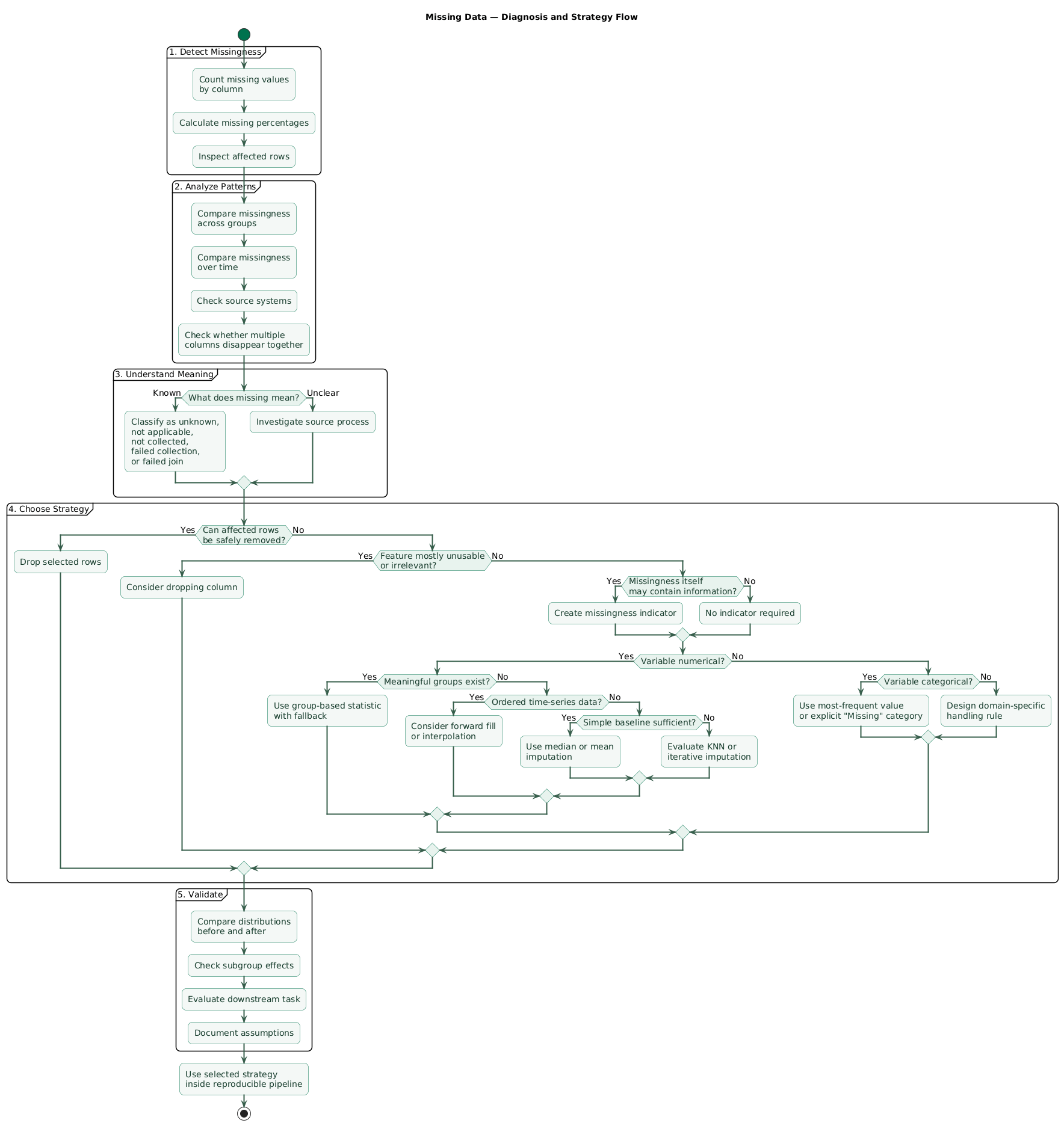
Count missing values
import pandas as pd

df = pd.read_csv("customers.csv")

missing_count = df.isna().sum()

missing_percent = (
    df.isna()
      .mean()
      .mul(100)
      .sort_values(ascending=False)
)

print(missing_count)
print(missing_percent)
Percentages make columns easier to compare, but the overall percentage is only the first step.
Look at patterns
Check whether missingness changes across:
- Time periods.
- Countries.
- Products.
- Device types.
- Customer segments.
- Data sources.
- Target classes.
missing_by_country = (
    df.groupby("country")["income"]
      .apply(lambda s: s.isna().mean())
      .sort_values(ascending=False)
)

print(missing_by_country)
If income is missing for 2% of customers in one country and 70% in another, global median imputation can hide an important data-collection difference.
Check whether columns disappear together
missing_pattern = df[
    ["income", "occupation", "employer"]
].isna().value_counts()

print(missing_pattern)
Multiple variables becoming missing simultaneously may reveal a form branch, source-system limitation, optional customer profile, or failed join.
Understand the meaning of null
Before filling a field, determine whether NaN means:
- Unknown.
- Not available yet.
- Not applicable.
- Not collected.
- Collection failed.
- Refused.
- No matching record existed.
Do not merge different meanings accidentally
“No spouse” and “spouse occupation unknown” are not the same state. Replacing both with one generic value can destroy useful information about the original process.
2. When dropping rows or columns is reasonable
Imputation is not mandatory. Sometimes deletion is simpler and more defensible.
Dropping rows may be reasonable when
- Only a very small fraction of observations is affected.
- The missingness does not appear concentrated in an important group.
- The dataset remains sufficiently large afterward.
- The missing record cannot support the intended analysis.
df_complete = df.dropna(
    subset=["target", "critical_measurement"]
)
Dropping a column may be reasonable when
- Almost all values are absent.
- The feature is not important to the analytical question.
- The field is unreliable or inconsistently collected.
- The remaining observed values are not representative enough to support useful inference.
Do not use a universal rule such as “drop every column above 40% missingness.” A field that is 80% missing may still contain high-value information for the 20% of records where it exists.
Measure what deletion changes
before = len(df)

reduced = df.dropna(subset=["income"])

after = len(reduced)

print("Rows removed:", before - after)
print("Percent removed:", (before - after) / before * 100)
Compare segment and target distributions before and after deletion. A small number of deleted rows can still introduce bias when they belong disproportionately to one group.
3. Simple numerical imputation: mean and median
Simple statistical imputation is often the best baseline because it is easy to understand, fast, reproducible, and difficult to misconfigure.
Median imputation with pandas
median_age = df["age"].median()

df["age_imputed"] = df["age"].fillna(median_age)
Mean imputation
mean_temperature = df["temperature"].mean()

df["temperature_imputed"] = (
    df["temperature"].fillna(mean_temperature)
)
Mean vs median
| Strategy | Useful when | Main limitation |
|---|---|---|
| Mean | Distribution is reasonably symmetric and mean is meaningful | Sensitive to extreme values |
| Median | Numerical variable is skewed or contains large valid extremes | Still collapses missing observations to one value |
Income, transaction amounts, house prices, and similar variables are often heavily skewed, making median imputation a practical first baseline.
SimpleImputer
from sklearn.impute import SimpleImputer

imputer = SimpleImputer(strategy="median")

X_imputed = imputer.fit_transform(
    df[["age", "income", "account_balance"]]
)
The important distinction is that fit() learns the
statistics and transform() applies them. That becomes crucial
when train and test data are separated.
Simple imputation changes the distribution
Replacing many missing observations with the same median creates an artificial concentration at that value and usually reduces variance. The method may still work well for prediction, but do not pretend that the completed column contains genuinely observed measurements.
4. Categorical imputation and explicit missing categories
Categorical variables require different assumptions than numerical ones.
Most-frequent category
from sklearn.impute import SimpleImputer

categorical_imputer = SimpleImputer(
    strategy="most_frequent"
)

X_category = categorical_imputer.fit_transform(
    df[["country", "subscription_type"]]
)
This can work when missingness is rare, but it hides the fact that the value was originally absent.
Explicit missing category
df["occupation"] = (
    df["occupation"]
      .fillna("Missing")
)
An explicit category can be especially useful when missingness has a meaningful operational interpretation.
categorical_imputer = SimpleImputer(
    strategy="constant",
    fill_value="Missing"
)
Be careful with semantic states
Consider a field named employment_status. A missing value
might mean the customer skipped the question. It should not automatically
become Unemployed, because that category has a completely
different meaning.
5. Preserve missingness with indicator features
Sometimes the fact that a value is missing predicts something important. An indicator feature preserves this signal while another strategy fills the original column.
Manual indicator
df["income_was_missing"] = (
    df["income"].isna().astype("int8")
)

df["income"] = df["income"].fillna(
    df["income"].median()
)
The model now receives both:
- A usable numerical value.
- A flag telling it whether that value was originally missing.
SimpleImputer with an indicator
from sklearn.impute import SimpleImputer

imputer = SimpleImputer(
    strategy="median",
    add_indicator=True
)

X_imputed = imputer.fit_transform(X)
Indicators are not automatically beneficial. Their value depends on whether the missingness process relates to the target or to important operational differences.
A practical baseline
For many tabular prediction tasks, median imputation plus missingness indicators is a useful baseline before testing more complicated imputation algorithms.
6. Group-based imputation
A single global median can be inappropriate when the expected value differs strongly between meaningful groups.
Imagine imputing employee salary. A global median ignores differences between job roles.
Group median with pandas
group_median = (
    df.groupby("job_role")["salary"]
      .transform("median")
)

df["salary_imputed"] = (
    df["salary"].fillna(group_median)
)
Add a fallback
Some groups may contain no observed values at all. Add a global fallback:
global_median = df["salary"].median()

group_median = (
    df.groupby("job_role")["salary"]
      .transform("median")
)

df["salary_imputed"] = (
    df["salary"]
      .fillna(group_median)
      .fillna(global_median)
)
Group imputation is appropriate when
- The grouping variable is known at inference time.
- The groups have genuine domain meaning.
- Groups contain enough observations for stable statistics.
- The grouping itself does not leak the target.
The same leakage rule still applies
For machine learning, group medians must be learned from the training partition rather than recalculated using the full dataset. Convenient pandas code written before the split can accidentally leak validation information.
7. Forward fill and interpolation for ordered data
Ordered measurements can support strategies that would be inappropriate for ordinary independent rows.
Forward fill
df = df.sort_values("timestamp")

df["status_ffill"] = df["status"].ffill()
Forward filling assumes the last observed state remains valid until a new measurement appears.
That may make sense for a configuration state or a slowly changing sensor setting. It may be completely wrong for rapidly changing measurements.
Limit long gaps
df["status_ffill"] = (
    df["status"].ffill(limit=2)
)
Limiting the number of propagated observations prevents one ancient value from being copied across a long period with no measurements.
Linear interpolation
df["temperature_interpolated"] = (
    df["temperature"].interpolate(
        method="linear"
    )
)
Time-aware interpolation
df = (
    df.set_index("timestamp")
      .sort_index()
)

df["temperature"] = (
    df["temperature"].interpolate(
        method="time"
    )
)
Interpolation estimates a value between observations. It is most defensible when measurements follow a meaningful ordered process and gaps are short relative to the dynamics being measured.
Do not interpolate arbitrary tabular rows
The row above and below a customer in a CSV file usually have no meaningful relationship. Interpolation only makes sense when ordering carries domain information.
8. KNN and iterative imputation
Python imputation strategy decision tree (diagram)
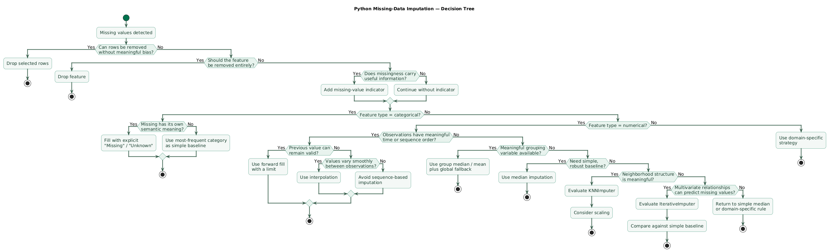
More complex imputation can use relationships between several features rather than filling every variable independently.
KNNImputer
K-nearest-neighbor imputation estimates a missing feature using nearby samples with available values.
from sklearn.impute import KNNImputer

imputer = KNNImputer(
    n_neighbors=5,
    weights="distance"
)

X_imputed = imputer.fit_transform(X)
KNN can be useful when
- Similar observations genuinely tend to have similar feature values.
- The dataset is not prohibitively large.
- The feature representation makes neighborhood distance meaningful.
Scaling matters
A feature measured in thousands can dominate a distance calculation over a feature ranging from zero to one. Think carefully about scaling and representation when using neighbor-based methods.
IterativeImputer
Iterative imputation treats each incomplete feature as a prediction problem using other features.
from sklearn.experimental import enable_iterative_imputer
from sklearn.impute import IterativeImputer

imputer = IterativeImputer(
    max_iter=10,
    random_state=42
)

X_imputed = imputer.fit_transform(X)
In current scikit-learn releases, IterativeImputer remains
experimental, so the explicit experimental import is still required.
Complex does not automatically mean better
Multivariate methods can preserve relationships better in some datasets, but they add:
- Computation.
- Hyperparameters.
- Modeling assumptions.
- Maintenance complexity.
- More opportunities for leakage.
Compare them with simple median, mode, or constant baselines rather than assuming advanced imputation must perform better.
9. Prevent train-test leakage with pipelines
One of the most important practical rules in imputation is:
Split first, learn imputation second
Do not calculate medians, means, neighbor relationships, category frequencies, or iterative-imputation models using the entire dataset before evaluating a machine-learning model.
The incorrect pattern
# Leakage: statistic sees all observations
df["income"] = df["income"].fillna(
    df["income"].median()
)

X_train, X_test, y_train, y_test = train_test_split(
    X, y, test_size=0.2, random_state=42
)
The median was calculated using records that later become part of the test set.
The correct pattern
from sklearn.model_selection import train_test_split
from sklearn.impute import SimpleImputer

X_train, X_test, y_train, y_test = train_test_split(
    X,
    y,
    test_size=0.2,
    random_state=42
)

imputer = SimpleImputer(strategy="median")

X_train_imputed = imputer.fit_transform(X_train)
X_test_imputed = imputer.transform(X_test)
The test data receives the training median. It does not influence the learned preprocessing rule.
Prefer a Pipeline
from sklearn.pipeline import Pipeline
from sklearn.impute import SimpleImputer
from sklearn.preprocessing import StandardScaler
from sklearn.linear_model import LogisticRegression

model = Pipeline([
    (
        "imputer",
        SimpleImputer(
            strategy="median",
            add_indicator=True
        )
    ),
    (
        "scaler",
        StandardScaler()
    ),
    (
        "classifier",
        LogisticRegression(max_iter=1000)
    )
])

model.fit(X_train, y_train)

score = model.score(X_test, y_test)
A pipeline applies the same learned preprocessing consistently during cross-validation, testing, and later inference.
Leakage-safe mixed-type preprocessing (diagram)

Different strategies for different columns
from sklearn.compose import ColumnTransformer
from sklearn.impute import SimpleImputer
from sklearn.preprocessing import OneHotEncoder
from sklearn.pipeline import Pipeline
from sklearn.linear_model import LogisticRegression

numeric_features = [
    "age",
    "income",
    "account_balance"
]

categorical_features = [
    "country",
    "subscription_type"
]

numeric_pipeline = Pipeline([
    (
        "imputer",
        SimpleImputer(
            strategy="median",
            add_indicator=True
        )
    )
])

categorical_pipeline = Pipeline([
    (
        "imputer",
        SimpleImputer(
            strategy="constant",
            fill_value="Missing"
        )
    ),
    (
        "encoder",
        OneHotEncoder(
            handle_unknown="ignore"
        )
    )
])

preprocessor = ColumnTransformer([
    (
        "numeric",
        numeric_pipeline,
        numeric_features
    ),
    (
        "categorical",
        categorical_pipeline,
        categorical_features
    )
])

model = Pipeline([
    ("preprocessor", preprocessor),
    (
        "classifier",
        LogisticRegression(max_iter=1000)
    )
])

model.fit(X_train, y_train)
This structure keeps learned preprocessing inside the same evaluation boundary as the predictive estimator.
10. Evaluate whether an imputation strategy is helping
Do not choose an imputer only because the completed dataset looks tidy. Evaluate the strategy in the context of the actual analytical task.
Compare simple baselines
For a numerical feature, compare:
- Median.
- Median + missing indicator.
- Group median where justified.
- KNN imputation.
- Iterative imputation.
Evaluate using cross-validation or another validation scheme appropriate to the data.
Artificial masking test
One way to compare reconstruction ability is to temporarily hide some known values, impute them, and compare estimates with the true values.
This does not perfectly reproduce naturally occurring missingness, but it can expose methods that perform particularly badly on your data.
Check downstream metrics
For machine learning, evaluate the final task:
- Classification metrics.
- Regression error.
- Calibration.
- Performance by important subgroup.
- Temporal validation performance.
Check stability
A complicated imputer that improves a validation metric by 0.1% but changes substantially between data batches may not justify the additional operational complexity.
Monitor production missingness
Record expected missing rates for important features. A change from 3% missing to 40% missing may indicate upstream pipeline failure even when the model continues accepting rows because the imputer hides the problem.
expected_max_missing = {
    "age": 0.05,
    "income": 0.20,
    "country": 0.02
}

for column, threshold in expected_max_missing.items():
    actual = df[column].isna().mean()

    if actual > threshold:
        print(
            f"WARNING: {column} missing rate "
            f"{actual:.1%} exceeds {threshold:.1%}"
        )
Imputation should not hide broken pipelines
A model can continue producing predictions after an upstream feature disappears entirely. Monitor missingness separately so successful technical imputation does not mask a data-quality incident.
11. Copy/paste missing-data checklist
Handling missing data in Python checklist

Understand missingness
- Count missing values by column.
- Calculate missing percentages.
- Inspect rows containing missing values.
- Compare missingness across categories.
- Compare missingness across data sources.
- Compare missingness across time.
- Compare missingness across target classes.
- Check whether multiple fields disappear together.
- Determine whether missing means unknown.
- Determine whether missing means not applicable.
- Determine whether missing means not collected.
- Determine whether missing means collection failure.
- Determine whether missing resulted from a failed join.
- Preserve the original missingness before transformation.

Before imputing
- Confirm the semantic type of each feature.
- Confirm units and ranges.
- Check for sentinel values such as -1, 999, or "unknown".
- Convert sentinel values to explicit missing values only when their meaning is confirmed.
- Decide whether the feature is available at inference time.
- Determine whether missingness itself may contain useful information.
- Document the proposed imputation assumption.

Deletion
- Measure how many rows would be removed.
- Check which segments would be disproportionately removed.
- Check whether target distribution changes after deletion.
- Consider dropping a feature only when its usefulness and available coverage justify it.
- Avoid universal missing-percentage rules without domain context.

Simple numerical imputation
- Establish a median baseline.
- Consider mean imputation for suitable symmetric variables.
- Remember that mean and median imputation reduce natural variance.
- Preserve an indicator when missingness may matter.
- Learn imputation statistics from training data only.

Categorical imputation
- Consider most-frequent imputation when missingness is rare.
- Consider an explicit "Missing" or "Unknown" category.
- Do not replace missing with an existing category that has a different semantic meaning.
- Check category cardinality after imputation.
- Ensure downstream encoders can handle categories not seen during training.

Missing indicators
- Test whether missingness predicts the target.
- Add explicit indicators where useful.
- Avoid automatically creating indicators for hundreds of unimportant features without evaluation.
- Keep indicator creation inside the preprocessing pipeline for predictive modeling.

Group-based imputation
- Use groups only when they have domain meaning.
- Ensure the grouping variable is available at inference time.
- Check group sample sizes.
- Add a fallback for groups with no observed values.
- Avoid target-derived grouping.
- Learn group statistics on training data only.

Time-series and ordered data
- Sort data before forward or backward filling.
- Confirm that row ordering has semantic meaning.
- Use forward fill only when the previous observation can reasonably remain valid.
- Limit propagation across long gaps.
- Use interpolation only for variables where values between observations are meaningful.
- Consider time-aware interpolation for irregular timestamps.
- Avoid interpolating arbitrary independent tabular rows.
- Prevent future observations from leaking into past predictions.

KNN imputation
- Establish a simple baseline first.
- Confirm that neighbor similarity has domain meaning.
- Consider feature scaling.
- Consider computational cost.
- Tune the number of neighbors using training data.
- Evaluate downstream model performance.

Iterative imputation
- Establish a simple baseline first.
- Understand that the method models incomplete features from other features.
- Use reproducible random-state settings where appropriate.
- Evaluate convergence and runtime.
- Prevent target or future information from entering the imputation model.
- Remember that scikit-learn IterativeImputer remains experimental.

Leakage prevention
- Split train and test data before learning imputation rules.
- Never calculate a global median on the full dataset before model evaluation.
- Fit imputers on training data only.
- Transform validation and test data with the fitted training imputer.
- Place preprocessing inside Pipeline where practical.
- Place column-specific transformations inside ColumnTransformer.
- Run cross-validation around the complete preprocessing pipeline.
- Keep target values out of feature imputation unless the statistical method explicitly requires and safely handles them.

Evaluation
- Compare against a simple baseline.
- Compare model performance across imputation strategies.
- Evaluate important subgroups separately.
- Use temporal validation when the production problem is temporal.
- Consider artificial masking experiments.
- Inspect the post-imputation distribution.
- Inspect changes in mean, median, variance, and quantiles.
- Check whether relationships between variables changed substantially.
- Document why the final strategy was selected.

Production monitoring
- Record expected missing rates.
- Alert on sudden missingness increases.
- Alert when an important feature becomes entirely missing.
- Monitor missingness by source system.
- Monitor missingness by time.
- Monitor missingness by customer segment.
- Version preprocessing pipelines.
- Store the fitted preprocessing configuration with the model.
- Reassess the strategy when upstream collection changes.

Final review
- Can you explain why each important field is missing?
- Can you explain why each imputation method was selected?
- Was every learned imputation parameter fitted on training data only?
- Does the model know when an important value was originally missing where needed?
- Did you compare the chosen strategy with a simpler baseline?
- Are missingness changes monitored after deployment?
12. FAQ
Should I always impute missing values?
No. Some observations can reasonably be removed, some features may be too unreliable to use, and some analytical methods can work with missing values directly. Missingness can also be informative. Diagnose the problem before selecting an imputation strategy.
Should I use mean or median imputation?
Median is often a practical baseline for skewed numerical variables because extreme observations affect it less. Mean imputation can be appropriate when the variable is reasonably symmetric and the mean has a useful interpretation. Both create artificial values and reduce natural variability.
When should I add a missing-value indicator?
Consider an indicator when the probability that a value is missing is related to the outcome or another meaningful process. It lets the model distinguish genuinely observed values from values inserted by an imputation step.
Is KNN imputation better than median imputation?
Not necessarily. KNN can exploit multivariate neighborhood structure, but it requires meaningful distance relationships and adds computational complexity. Compare it against median imputation using an appropriate validation procedure.
When should I use interpolation?
Use interpolation when observations have a meaningful order and values between known measurements can reasonably be estimated from neighboring observations. Time-series sensor measurements are a common example. Arbitrary neighboring rows in a normal tabular dataset are not.
How does imputation cause data leakage?
Leakage occurs when information from validation or test observations influences the imputer. A median calculated from the entire dataset, for example, contains information from the future test partition. Split first and fit the imputer only on training data.
Key terms (quick glossary)
- Missing value
-
An absent observation represented by a marker such as
NaN,None, or another explicitly defined missing-value representation. - Imputation
- Replacing a missing value with an estimated, derived, or explicitly chosen replacement so the data can be used by downstream analysis.
- Mean imputation
- Replacing missing numerical values with the arithmetic mean calculated from observed training values.
- Median imputation
- Replacing missing numerical values with the median of observed training values, often providing a robust simple baseline for skewed features.
- Mode imputation
- Replacing missing values with the most frequently observed value or category.
- Missingness indicator
- A binary feature recording whether the corresponding original value was missing before imputation.
- Forward fill
- Filling a missing observation with the most recent preceding observed value in an ordered dataset.
- Interpolation
- Estimating missing values from neighboring observations according to a mathematical or time-aware relationship.
- KNN imputation
- A multivariate method that estimates missing values using observations considered similar according to a nearest-neighbor distance.
- Iterative imputation
- A multivariate approach that repeatedly models incomplete features using other available features.
- Data leakage
- Information entering preprocessing or modeling that would not be legitimately available when the system makes predictions in real use.
- Pipeline
- A reproducible sequence of preprocessing and modeling steps fitted and applied together, helping ensure transformations use the correct training-data boundary.
Worth reading
Recommended guides from the category.