Feature Engineering for Tabular Data: Simple Techniques That Win Baselines

Feature engineering is often described as inventing complicated transformations. In tabular machine learning, some of the most useful features are much simpler: account age instead of a raw signup date, price per item instead of price and quantity viewed independently, a missing-value flag, or historical transaction counts instead of thousands of raw events.

The objective is not to create as many columns as possible. It is to represent useful structure in a form the model can learn efficiently.

A strong workflow starts with a reproducible baseline and adds one defensible idea at a time. That makes improvements measurable and prevents a feature-engineering notebook from becoming an undocumented collection of transformations.

1. Start with a real baseline before engineering features

Tabular feature-engineering workflow (diagram)

Without a baseline, you cannot tell whether feature engineering actually helped.

A baseline should include

• A fixed validation strategy.
• A simple preprocessing pipeline.
• A reasonable baseline model.
• A clearly defined evaluation metric.
• Reproducible random seeds where relevant.

For mixed tabular data, a baseline might use median imputation for numeric columns, explicit missing categories plus one-hot encoding for categorical columns, and a regularized linear model or a tree-based estimator.

Keep the validation scheme fixed

If feature A is evaluated with one split and feature B with another, the difference may come from the split instead of the feature.

Use the same folds or the same train-validation boundary when comparing transformations.

Track incremental experiments

experiment                         cv_auc
------------------------------------------------
raw_baseline                       0.781
+ date_features                    0.794
+ log_revenue                      0.798
+ customer_activity_ratio          0.806
+ random_polynomials               0.801

The final line is important. More features can make the model worse.

2. Convert raw columns into domain meaning

The highest-value feature engineering often comes from asking what each raw field represents.

Suppose a customer table contains:

signup_date
last_login_date
total_orders
total_revenue
support_tickets
subscription_price

The raw values are usable, but several derived concepts may be closer to the actual behavior you want the model to learn.

account_age_days
days_since_last_login
average_order_value
orders_per_month
support_tickets_per_order
revenue_per_month

Ask four questions for every important column

1. Is the absolute value meaningful?
2. Would a relative value be more meaningful?
3. Does time change its interpretation?
4. Is the feature really a proxy for another business concept?

Example: account age

A signup timestamp is usually less directly useful than the duration between signup and prediction time.

prediction_date = pd.Timestamp("2026-08-20")

df["account_age_days"] = (
    prediction_date - df["signup_date"]
).dt.days

For historical model training, use the prediction timestamp associated with each row rather than one global present-day date.

3. Log transforms, ratios, differences, and rates

Logarithmic transforms

Many real-world numerical features have long right tails:

• Revenue.
• Income.
• Transaction amount.
• Page views.
• Customer lifetime value.
• File size.

A logarithmic transform can compress the extreme tail and make relative differences more prominent.

import numpy as np

df["revenue_log1p"] = np.log1p(
    df["total_revenue"]
)

log1p(x) computes the logarithm of 1 + x, which is convenient for non-negative variables containing zeros.

Do not apply it automatically to variables that contain invalid negative values or where the original scale is already appropriate.

Ratios

Ratios express relative behavior that two raw values may hide.

df["average_order_value"] = (
    df["total_revenue"]
    / df["total_orders"].replace(0, np.nan)
)

Other examples:

clicks / impressions
late_payments / invoices
support_tickets / active_months
used_storage / storage_limit
completed_tasks / assigned_tasks

Protect division by zero

A denominator of zero usually has business meaning. Decide whether the resulting ratio should be missing, zero, capped, or represented by an additional flag.

Differences

Sometimes the gap matters more than either raw quantity.

df["price_discount"] = (
    df["list_price"] - df["sale_price"]
)

df["balance_change"] = (
    df["current_balance"] - df["previous_balance"]
)

Rates

df["orders_per_active_month"] = (
    df["total_orders"]
    / df["active_months"].clip(lower=1)
)

Rates make entities with different exposure periods more comparable.

4. Extract useful information from dates and time

Raw timestamps contain multiple possible signals. Decompose only those that make sense for the problem.

df["created_at"] = pd.to_datetime(
    df["created_at"],
    utc=True
)

df["year"] = df["created_at"].dt.year
df["month"] = df["created_at"].dt.month
df["weekday"] = df["created_at"].dt.dayofweek
df["hour"] = df["created_at"].dt.hour
df["is_weekend"] = (
    df["created_at"].dt.dayofweek >= 5
).astype("int8")

Useful date-derived features include

• Year.
• Month.
• Day of week.
• Hour.
• Weekend indicator.
• Quarter.
• Days since registration.
• Days since last activity.
• Duration between two events.

Cyclical features

Month 12 and month 1 are numerically far apart but temporally adjacent. The same issue appears with hour 23 and hour 0.

df["month_sin"] = np.sin(
    2 * np.pi * df["month"] / 12
)

df["month_cos"] = np.cos(
    2 * np.pi * df["month"] / 12
)

Sine and cosine features can make periodic structure easier for models that do not automatically infer circular relationships.

Tree models may need less transformation

Tree-based models can learn thresholds from raw month or hour values, but explicit cyclic or domain-derived features can still help when the relationship wraps around or when the feature expresses useful prior knowledge.

5. Make categorical variables easier to learn

Normalize categories before encoding

Fix known semantic duplicates first.

country_map = {
    "United States": "US",
    "USA": "US",
    "U.S.A.": "US",
    "us": "US"
}

df["country_clean"] = (
    df["country"]
      .str.strip()
      .replace(country_map)
)

One-hot encoding

One-hot encoding is a strong baseline for low- and moderate-cardinality nominal features.

from sklearn.preprocessing import OneHotEncoder

encoder = OneHotEncoder(
    handle_unknown="ignore"
)

Unknown-category handling matters because production may contain a category that never appeared during training.

Group rare categories

A feature with hundreds or thousands of rare values can create a very wide sparse feature matrix.

One approach is to map categories below a training-frequency threshold to an Other category.

Modern one-hot encoders can also group infrequent categories through frequency or category-count controls.

Frequency features

The training frequency of a category can sometimes be informative.

frequency = (
    X_train["merchant"]
      .value_counts(normalize=True)
)

X_train["merchant_frequency"] = (
    X_train["merchant"].map(frequency)
)

X_valid["merchant_frequency"] = (
    X_valid["merchant"]
      .map(frequency)
      .fillna(0)
)

6. Turn missingness into a feature when it matters

A missing value can encode a real process: a customer skipped a question, one data source does not collect the field, or a measurement fails for a particular device type.

df["income_missing"] = (
    df["income"].isna().astype("int8")
)

You can then impute the original field while preserving the information that the original value was absent.

df["income"] = (
    df["income"]
      .fillna(df["income"].median())
)

Useful missing indicators often involve

• Income.
• Optional profile fields.
• Sensor measurements.
• Credit or risk attributes.
• Incomplete historical records.

Do not create hundreds of missing indicators automatically unless you validate whether they improve the model.

7. Add interactions instead of blindly adding complexity

Feature-engineering decision tree (diagram)

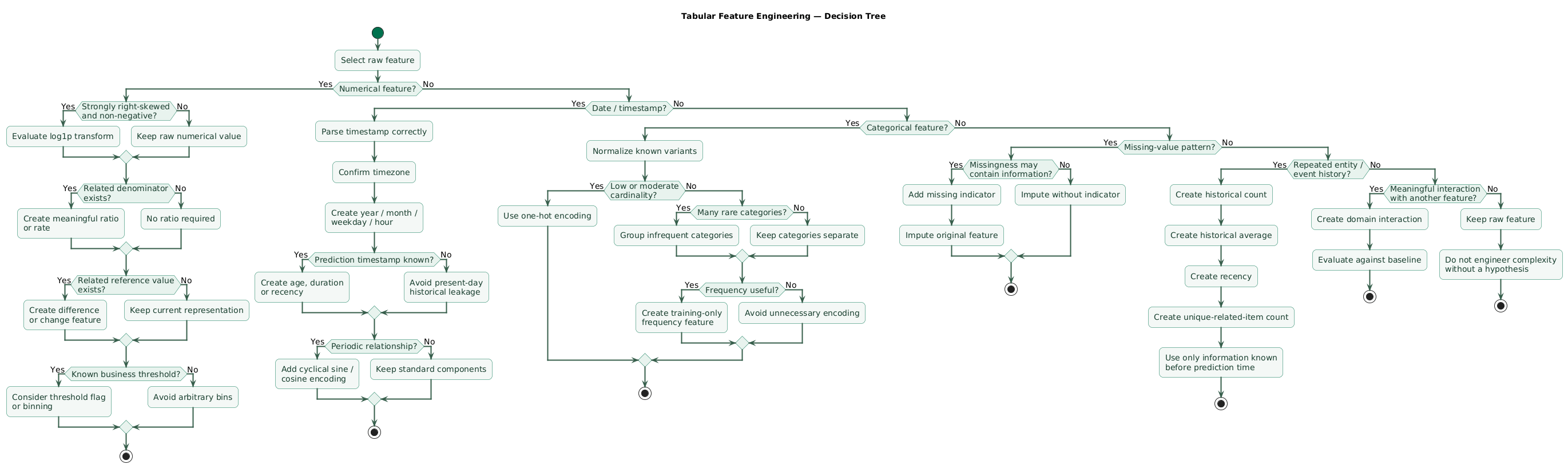
An interaction represents the idea that the effect of one variable depends on another.

Manual interaction

df["price_x_quantity"] = (
    df["price"] * df["quantity"]
)

That example has an obvious interpretation: total value.

Another example

df["usage_per_user"] = (
    df["monthly_usage"]
    / df["active_users"].clip(lower=1)
)

PolynomialFeatures

For a small set of numerical features and a model that cannot easily discover interactions itself, polynomial features can generate products and higher-order terms.

from sklearn.preprocessing import PolynomialFeatures

poly = PolynomialFeatures(
    degree=2,
    include_bias=False
)

X_poly = poly.fit_transform(
    X[["age", "income", "balance"]]
)

The number of generated features grows quickly, so avoid applying polynomial expansion indiscriminately to a large table.

Tree models already learn many interactions

Decision trees and tree ensembles naturally split on combinations of features, so generic polynomial expansion is usually less attractive for them.

Domain interactions can still help because they compress several raw columns into a meaningful concept such as utilization, margin, account age, or customer activity.

8. Group and historical aggregate features

For transaction, event, or repeated-entity datasets, aggregates can be among the strongest features.

Suppose each row is a transaction. Useful customer-level historical features might include:

• Number of previous transactions.
• Average previous transaction amount.
• Maximum previous transaction amount.
• Days since previous transaction.
• Number of merchants used.
• Fraction of transactions occurring at night.

Static aggregate example

customer_stats = (
    transactions
      .groupby("customer_id")
      .agg(
          order_count=("order_id", "count"),
          average_order=("amount", "mean"),
          max_order=("amount", "max")
      )
)

This is appropriate only when the complete aggregation window is legitimately available for the prediction being made.

Historical aggregate

For temporal predictions, calculate only information from previous rows.

transactions = transactions.sort_values(
    ["customer_id", "timestamp"]
)

transactions["previous_order_count"] = (
    transactions
      .groupby("customer_id")
      .cumcount()
)

Historical expanding mean

transactions["previous_average_amount"] = (
    transactions
      .groupby("customer_id")["amount"]
      .transform(
          lambda s: s.shift(1).expanding().mean()
      )
)

The shift prevents the current transaction from contributing to its own historical feature.

Target-dependent group aggregates

Be especially careful with features such as average target value by category. These are forms of target encoding and require fold-aware calculations so validation labels do not influence validation features.

9. Binning and threshold-style features

Binning converts a continuous variable into intervals.

df["age_band"] = pd.cut(
    df["age"],
    bins=[0, 18, 30, 45, 65, 120],
    labels=[
        "under_18",
        "18_29",
        "30_44",
        "45_64",
        "65_plus"
    ]
)

Binning can help when

• Business decisions already use thresholds.
• The relationship is strongly nonlinear.
• A linear model needs more flexibility.
• Interpretability matters.

Quantile-based bins

df["income_quantile"] = pd.qcut(
    df["income"],
    q=5,
    duplicates="drop"
)

Quantile thresholds are learned from data, so in a predictive workflow they belong inside the training boundary.

KBinsDiscretizer

from sklearn.preprocessing import KBinsDiscretizer

binner = KBinsDiscretizer(
    n_bins=5,
    encode="onehot",
    strategy="quantile"
)

Binning can increase flexibility for a linear model but can also throw away useful numerical ordering or create unstable boundaries. Compare it against the raw numerical feature rather than assuming it is superior.

10. Keep feature engineering leakage-safe

Leakage-safe feature-engineering pipeline (diagram)

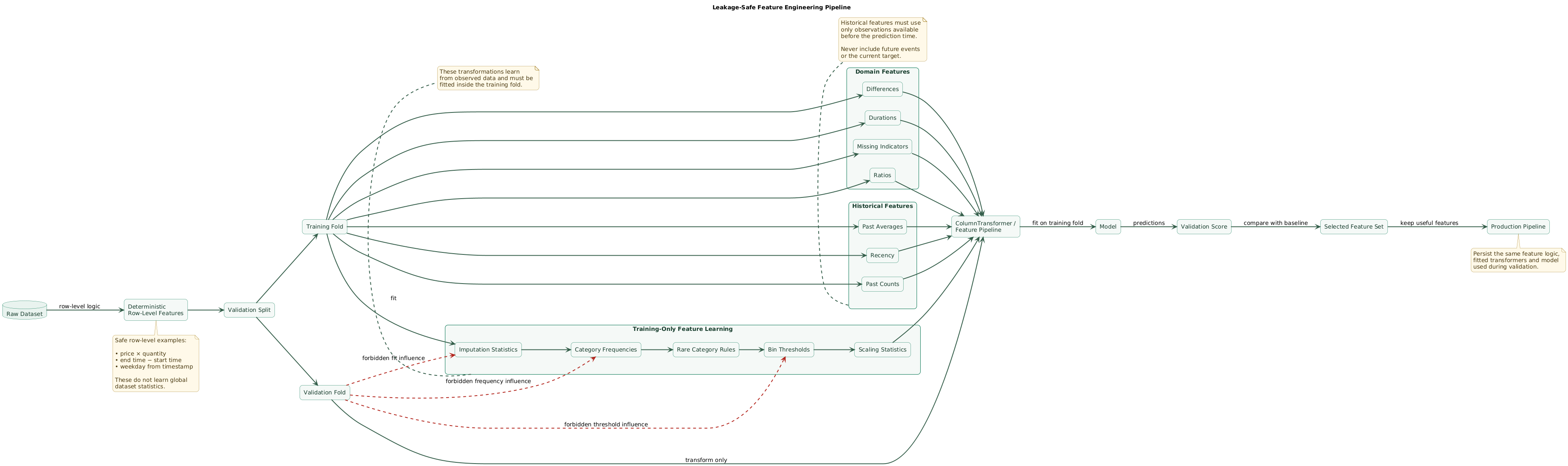
Feature engineering can leak information just as easily as preprocessing.

Usually safe before splitting

Deterministic row-level transformations that use only information already present in that row and do not learn from the full dataset can often be defined before splitting.

Examples:

total_price = quantity * unit_price

duration = end_time - start_time

is_weekend = weekday in [5, 6]

Must usually learn from training data only

• Median or mean values.
• Scaling statistics.
• Category frequency tables.
• Quantile thresholds.
• Rare-category thresholds based on observed frequency.
• Feature-selection decisions.
• PCA.
• Target encoding.
• Group aggregates that include held-out observations.

ColumnTransformer baseline

from sklearn.compose import ColumnTransformer
from sklearn.impute import SimpleImputer
from sklearn.preprocessing import OneHotEncoder
from sklearn.preprocessing import StandardScaler
from sklearn.pipeline import Pipeline
from sklearn.linear_model import LogisticRegression

numeric_features = [
    "age",
    "account_age_days",
    "revenue_log1p",
    "average_order_value"
]

categorical_features = [
    "country",
    "plan",
    "signup_month"
]

numeric_pipeline = Pipeline([
    (
        "imputer",
        SimpleImputer(
            strategy="median",
            add_indicator=True
        )
    ),
    (
        "scaler",
        StandardScaler()
    )
])

categorical_pipeline = Pipeline([
    (
        "imputer",
        SimpleImputer(
            strategy="constant",
            fill_value="Missing"
        )
    ),
    (
        "encoder",
        OneHotEncoder(
            handle_unknown="ignore"
        )
    )
])

preprocessor = ColumnTransformer([
    (
        "numeric",
        numeric_pipeline,
        numeric_features
    ),
    (
        "categorical",
        categorical_pipeline,
        categorical_features
    )
])

model = Pipeline([
    ("preprocessor", preprocessor),
    (
        "classifier",
        LogisticRegression(
            max_iter=1000
        )
    )
])

This keeps learned preprocessing inside the model-selection workflow.

Use ablation testing

An ablation test removes one feature or feature group and measures the effect.

baseline
baseline + date features
baseline + ratio features
baseline + date + ratio features
baseline + all engineered features

This tells you whether the feature really adds value or simply accompanies another useful transformation.

Do not judge features only by feature importance

A feature can appear highly important while being unstable, redundant, or leaky. Conversely, several individually modest features can improve the model together.

Prefer reproducible feature functions

def add_domain_features(df):
    out = df.copy()

    out["revenue_log1p"] = np.log1p(
        out["total_revenue"].clip(lower=0)
    )

    out["average_order_value"] = (
        out["total_revenue"]
        / out["total_orders"].replace(0, np.nan)
    )

    out["income_missing"] = (
        out["income"].isna().astype("int8")
    )

    return out

Avoid manually creating a column in a notebook and forgetting to reproduce the exact logic during inference.

Monitor engineered features in production

A derived feature can fail even when the raw input schema still looks valid.

Monitor:

• Missing rates.
• Minimum and maximum.
• Quantiles.
• Frequency of categories.
• Division-by-zero rates.
• Unexpected infinities.
• Distribution drift.

11. Copy/paste feature-engineering checklist

Tabular feature-engineering checklist

Baseline
- Define the production prediction task.
- Choose the validation strategy first.
- Build a simple reproducible baseline.
- Record the baseline metric.
- Keep validation folds fixed while comparing features.
- Track every feature experiment.

Raw feature review
- Define the meaning of each important column.
- Confirm the unit of each numerical variable.
- Confirm the semantic type of each column.
- Identify IDs that should not be treated as continuous numbers.
- Identify date and timestamp columns.
- Identify repeated entities.
- Identify potentially leaky post-outcome variables.

Numerical features
- Inspect numerical distributions.
- Consider log1p for strongly right-skewed non-negative features.
- Compare raw and transformed versions.
- Create meaningful differences.
- Create ratios where relative scale matters.
- Create rates where exposure time or opportunity differs.
- Protect divisions from zero denominators.
- Check generated infinities.
- Check unreasonable extreme values.
- Preserve interpretable raw features when useful.

Dates and time
- Parse timestamps explicitly.
- Normalize timezone assumptions.
- Extract useful year, month, weekday, or hour features.
- Add weekend or business-hour flags when relevant.
- Create durations between meaningful events.
- Create account or object age as of prediction time.
- Create recency features such as days since last event.
- Consider cyclical sine/cosine representations.
- Avoid calculating durations using information after prediction time.

Categorical features
- Normalize whitespace.
- Normalize known spelling variants.
- Merge categories only with a documented semantic mapping.
- Use one-hot encoding as a baseline for manageable cardinality.
- Handle unknown production categories.
- Consider grouping infrequent categories.
- Consider frequency features for high-cardinality variables.
- Learn category frequency mappings from training data only.
- Avoid treating arbitrary category IDs as meaningful continuous numbers.

Missing values
- Diagnose why values are missing.
- Consider a missing indicator when absence carries information.
- Keep imputation inside the training boundary.
- Avoid replacing missing values with a category that means something different.
- Monitor missingness after deployment.

Interactions
- Create interactions with domain meaning first.
- Consider price times quantity.
- Consider utilization or percentage features.
- Consider activity per unit of exposure.
- Consider differences between related measurements.
- Use PolynomialFeatures only on a controlled subset.
- Avoid combinatorial feature explosion.
- Remember that tree models can learn many interactions automatically.

Group aggregates
- Identify repeated entity IDs.
- Consider historical event counts.
- Consider historical means and medians.
- Consider historical maxima and minima.
- Consider recency since the previous event.
- Consider number of unique related entities.
- Use past-only aggregates for temporal prediction.
- Shift rolling or expanding features when necessary.
- Never allow the current target to influence its own aggregate.
- Fit validation-sensitive aggregate mappings inside training folds.

Binning
- Consider business-defined threshold bins.
- Consider discretization for strongly nonlinear relationships.
- Compare binned and continuous versions.
- Learn quantile bin boundaries from training data only.
- Avoid excessive numbers of bins.
- Check whether bin boundaries are stable across folds.

Feature selection
- Do not select features on the complete dataset before cross-validation.
- Evaluate engineered features with the same validation scheme.
- Remove features that add complexity without reliable improvement.
- Check correlated and redundant features.
- Investigate suspiciously predictive features for leakage.
- Use ablation tests to measure feature contribution.

Leakage
- Confirm every feature exists at prediction time.
- Remove post-outcome information.
- Prevent future observations from entering historical features.
- Split before learning dataset-level statistics.
- Fit frequency mappings on training data only.
- Fit bin thresholds on training data only.
- Fit scalers and imputers on training data only.
- Keep target encoding fold-aware.
- Keep feature selection inside cross-validation.
- Keep grouped entities separated where required.

Pipelines
- Put learned preprocessing inside Pipeline.
- Use ColumnTransformer for mixed column types.
- Keep encoding inside the pipeline.
- Keep imputation inside the pipeline.
- Keep scaling inside the pipeline.
- Keep automated feature selection inside the pipeline.
- Persist the complete fitted preprocessing and model workflow.

Evaluation
- Compare every feature group against the baseline.
- Use cross-validation where appropriate.
- Review mean validation performance.
- Review fold-to-fold variability.
- Review important subgroups.
- Review temporal performance where relevant.
- Reject improvements that disappear across folds.
- Prefer simple stable gains over fragile complexity.

Production
- Reproduce the same feature code during inference.
- Version feature definitions.
- Test feature generation on unseen categories.
- Test division-by-zero cases.
- Test missing input.
- Test extreme numerical input.
- Monitor feature missingness.
- Monitor feature distributions.
- Monitor category frequencies.
- Monitor unexpected infinities.
- Monitor feature drift.
- Remove obsolete features when they are no longer used.

Final review
- Can every engineered feature be explained in one sentence?
- Is every feature available at real prediction time?
- Does the feature improve validation reliably?
- Is the feature reproducible?
- Does its complexity justify its value?
- Can the production system calculate it consistently?

12. FAQ

What feature engineering should I try first on tabular data?

Start with features that express obvious domain structure: durations, date components, ratios, differences, rates, log transforms for heavily skewed positive variables, missing indicators, clean categorical encoding, and a small number of meaningful interactions.

Do tree-based models still need feature engineering?

Yes, although usually less generic numerical transformation is required. Trees can learn thresholds and many interactions directly, but they still benefit from domain information such as account age, historical counts, ratios, recency, normalized categories, and features that are not recoverable from a single raw column.

Should I one-hot encode every categorical feature?

No. One-hot encoding is a strong baseline for manageable cardinality. Very high-cardinality columns can produce large sparse feature spaces and may benefit from rare-category grouping, frequency representations, hashing, native categorical handling, or carefully validated target-based approaches.

Are polynomial features useful for tabular data?

They can be useful for linear models when a small number of numerical features have nonlinear or interaction effects. Apply them selectively. Polynomial expansion across dozens of columns can create an unnecessarily large feature space.

Can feature engineering cause data leakage?

Yes. Category frequencies, group aggregates, bin thresholds, target encoding, feature selection, and historical calculations can leak held-out or future information. Fit learned transformations inside the training boundary and calculate temporal features using only information available before prediction time.

How do I know whether an engineered feature is useful?

Compare the model with and without the feature using the same validation scheme. Check average performance, fold stability, important subgroups, production availability, and operational complexity. Keep features that provide repeatable value.

Key terms (quick glossary)

Feature engineering

The process of transforming raw data into variables that expose useful structure to a statistical or machine-learning model.

Baseline

A simple reproducible model and feature set used as the reference point for evaluating later improvements.

Interaction feature

A feature representing the combined effect of two or more variables, such as price multiplied by quantity.

Ratio feature

A feature formed by dividing one quantity by another to represent relative scale, efficiency, utilization, or rate.

Log transform

A nonlinear transformation that compresses large positive values and can make heavily skewed numerical distributions easier to model.

Cyclical encoding

A representation, commonly using sine and cosine, that preserves the circular relationship of periodic values such as hour, weekday, or month.

One-hot encoding

A categorical representation that creates a binary feature for each encoded category.

Frequency encoding

Representing a category using how frequently it appears in the training data.

Aggregate feature

A summary created from multiple related observations, such as previous transaction count or historical average purchase value.

Discretization

Converting a continuous numerical feature into intervals or bins.

Ablation test

An experiment in which one feature or feature group is removed to measure how much it contributes to model performance.

Feature leakage

The use of information in a feature that would not legitimately be available when the production prediction is made.