A/B Testing with Small Traffic: Designing Experiments You Can Trust

Low traffic does not make randomized experiments impossible. It makes careless experiments expensive.

When millions of users enter an experiment every day, a badly chosen metric or inefficient design may still accumulate enough observations to detect a useful effect. A small website, SaaS product, newsletter, internal tool, or niche marketplace does not have that luxury.

Every observation needs to answer a well-defined question. The experiment should target an effect worth acting on, avoid unnecessary variants and metrics, preserve clean randomization, and stop only according to a statistical procedure chosen before the results become tempting.

1. Small traffic changes the experiment you can afford

Small-traffic experiment design flow (diagram)

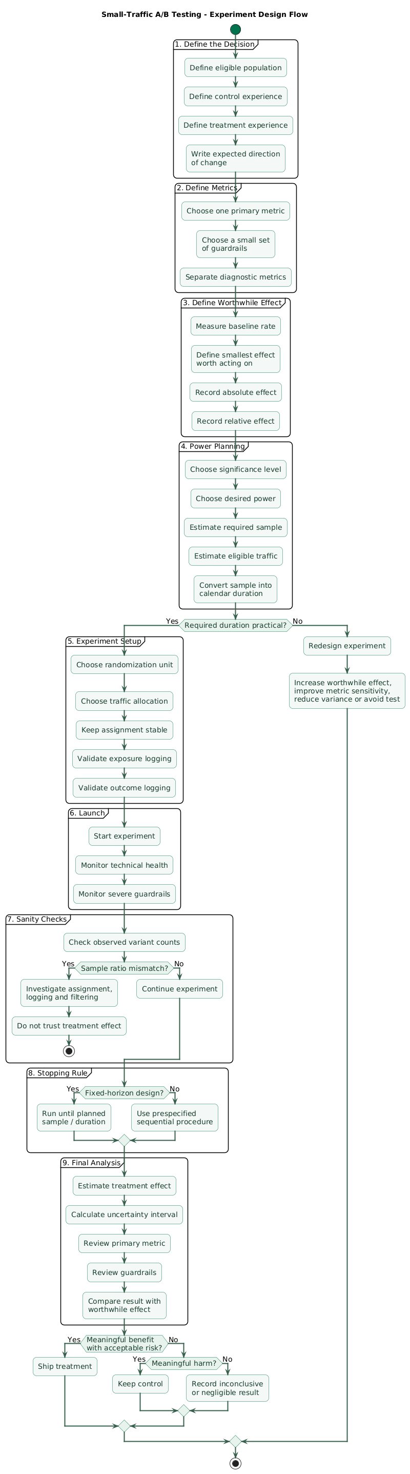
The main limitation in a small experiment is statistical information. Noisy metrics and tiny treatment effects require more observations.

That creates a fundamental tradeoff:

smaller effect you want to detect
              ↓
more observations required
              ↓
longer experiment duration

If you receive 400 eligible users per week, an experiment requiring 30,000 users is not a six-week project. It is a design warning.

There are four useful responses

• Test a larger change with a larger plausible effect.
• Use a more sensitive metric.
• Reduce avoidable variance.
• Decide that an A/B test is not the right tool for this decision.

What you should not do is launch an underpowered experiment and then wait until noise happens to produce an attractive result.

2. Write the decision before calculating sample size

Start with a product hypothesis rather than with the statistical test.

Weak experiment statement

Let's test the new checkout.

Better experiment statement

For eligible checkout users,
showing the shorter checkout flow
is expected to increase completed purchases
without materially increasing refunds
or payment failures.

The second version identifies:

• The eligible population.
• The treatment.
• The expected direction.
• The primary outcome.
• Potential guardrail failures.

Predefine the decision

Write down what would happen for each plausible result:

Clear meaningful improvement:
ship treatment.

Clear meaningful harm:
keep control.

Estimate near zero with narrow uncertainty:
treatment probably not worth shipping.

Very wide uncertainty:
experiment was inconclusive.

“Inconclusive” is a legitimate result. It is better than pretending an underpowered test proved that the variants are equivalent.

3. Choose a minimum detectable effect that actually matters

The minimum detectable effect, or MDE, is the treatment difference you design the experiment to detect with a chosen statistical power and significance level.

The important word is minimum. It should not be selected only because a sample-size calculator produces a convenient number.

Start from the business decision

Suppose checkout conversion is currently 8%.

Your team may decide that a move from 8.0% to 8.1% is too small to justify implementation and maintenance cost, while 8.0% to 8.8% would clearly be valuable.

The second difference is:

absolute effect:
8.8% - 8.0% = 0.8 percentage points

relative effect:
(8.8% - 8.0%) / 8.0% = 10%

MDE is not the observed result

MDE is a design input. The final experiment should still report the observed effect and its uncertainty rather than claiming that the true effect equals the MDE.

4. Estimate power, sample size, and realistic duration

Traffic, effect size, and experiment duration (diagram)

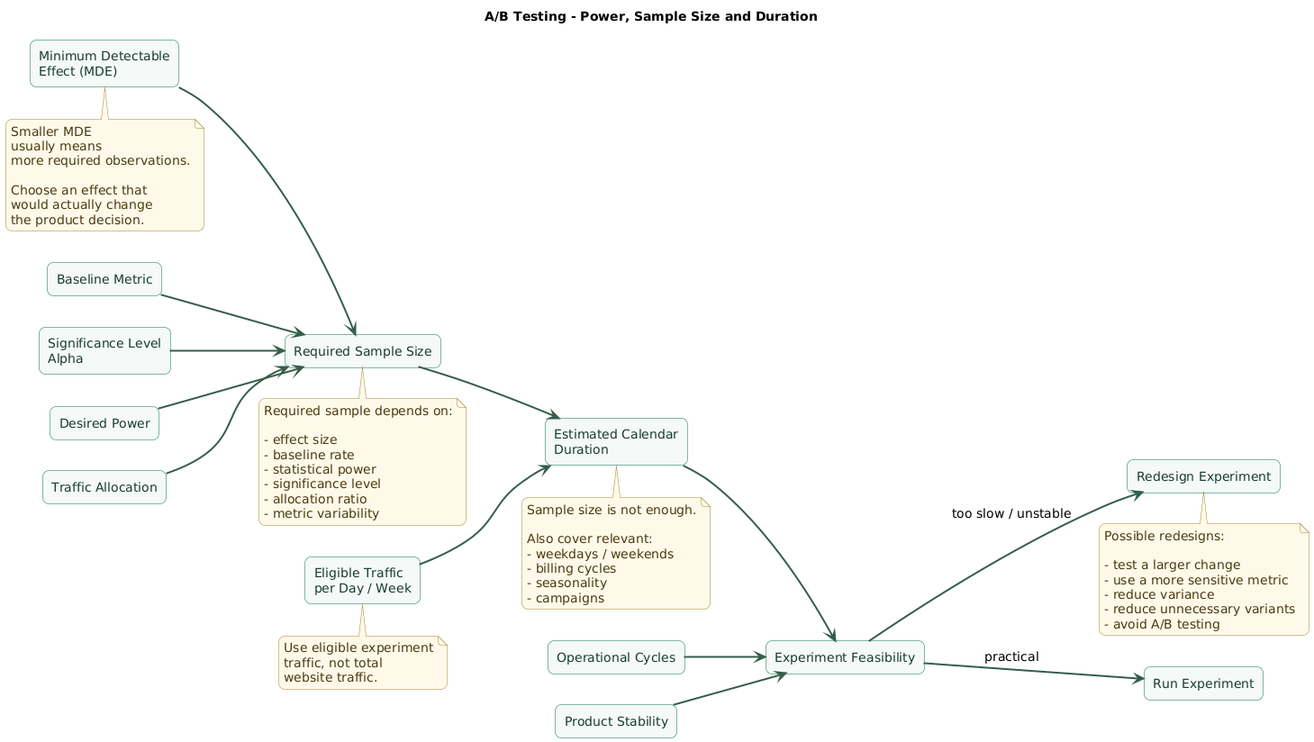
Power is the probability that the statistical procedure rejects the null hypothesis when the specified alternative effect is actually present.

Common design inputs include:

• Baseline conversion rate.
• Minimum detectable effect.
• Significance level.
• Desired power.
• Traffic allocation.

Example with statsmodels

The following example asks how many observations per variant are needed for a two-sided comparison of two conversion proportions.

from statsmodels.stats.proportion import (
    power_proportions_2indep
)

baseline = 0.08
target = 0.088
difference = target - baseline

alpha = 0.05
required_power = 0.80

n_per_variant = None

for n in range(100, 200_001):
    result = power_proportions_2indep(
        diff=difference,
        prop2=baseline,
        nobs1=n,
        ratio=1,
        alpha=alpha,
        alternative="two-sided"
    )

    if result.power >= required_power:
        n_per_variant = n
        break

print(n_per_variant)

Use the result as a planning estimate based on the assumptions supplied. Real data can differ from the baseline used in the calculation.

Convert sample size into calendar duration

total_required = 2 * n_per_variant

eligible_users_per_day = 250

estimated_days = (
    total_required / eligible_users_per_day
)

print(estimated_days)

Do not use total website traffic when only a subset of visitors can enter the experiment.

Calendar duration still matters

A sample-size calculation does not understand:

• Weekday vs weekend behavior.
• Monthly billing cycles.
• Marketing campaigns.
• Seasonal demand.
• Paydays.
• Product releases.

An experiment that reaches the nominal sample in two unusually busy days may not represent normal behavior. Plan enough calendar coverage to represent the operational cycle relevant to your product.

Do not reduce the sample requirement by pretending the MDE is larger

A larger assumed MDE reduces the required sample because the test is explicitly giving up sensitivity to smaller effects.

That is valid only when those smaller effects genuinely would not change the decision.

5. Randomize the right unit and keep assignment stable

Randomization is what gives the experiment its causal interpretation.

Choose the randomization unit

Possible units include:

• User.
• Account.
• Organization.
• Device.
• Session.

The correct unit depends on how treatment is experienced.

Example: user vs session

If a visitor sees checkout A in one session and checkout B the next day, behavior can be contaminated by prior exposure.

Stable user-level assignment is usually preferable when users return and treatment changes their ongoing experience.

Keep related users together when treatment spills over

In a collaboration product, treating half the members of one organization may affect untreated colleagues.

In that case, organization-level randomization may better represent the intervention, although having fewer independent organizations can sharply reduce effective statistical power.

Prefer efficient allocation when risk allows

For a simple two-arm experiment with similar measurement variance and symmetric statistical objectives, approximately equal allocation usually uses observations efficiently.

A risky treatment may still begin at lower exposure for safety and later ramp to a broader allocation after basic sanity checks.

6. Use one primary metric and a small guardrail set

Small experiments cannot afford an uncontrolled metric fishing expedition.

Primary metric

Choose one metric that best represents the hypothesis.

Examples:

• Checkout completion rate.
• Trial activation rate.
• Successful task completion.
• Revenue per eligible user.

Guardrail metrics

Guardrails protect against shipping a treatment that improves the primary metric by harming something critical.

Examples:

• Error rate.
• Payment failure rate.
• Refund rate.
• Latency.
• Unsubscribe rate.

Avoid dozens of primary outcomes

Testing many metrics and reporting only those that happen to move creates a multiple-comparison problem and encourages post-hoc storytelling.

Pre-label metrics:

primary:
purchase_conversion

guardrails:
payment_failure_rate
refund_rate

diagnostic:
checkout_step_1
checkout_step_2
checkout_step_3

Diagnostic metrics can explain a result without becoming independent excuses to declare the experiment successful.

7. Check sample ratio mismatch before trusting results

Suppose you configured a 50/50 split but observe:

Control:   5,400 users
Treatment: 4,600 users

The first question should not be which variant converted better. It should be why assignment or measurement differs from the expected ratio.

Possible SRM causes

• Broken randomization.
• Treatment-specific logging failures.
• Variant-specific redirects.
• Filtering after treatment exposure.
• Bot filtering that affects one variant differently.
• Missing telemetry.
• Users becoming eligible differently after assignment.

Simple chi-square sanity check

from scipy.stats import chisquare

observed = [5400, 4600]
expected = [5000, 5000]

statistic, p_value = chisquare(
    observed,
    f_exp=expected
)

print(statistic)
print(p_value)

The purpose is not to mechanically apply one universal p-value threshold. Treat an unexpected allocation as a data-quality signal and diagnose the experiment pipeline before interpreting treatment effects.

8. Do not turn daily peeking into a stopping rule

Teams naturally want to open the dashboard every morning.

Monitoring for technical failures and severe guardrail regressions is useful. Repeatedly asking whether a conventional fixed-horizon p < 0.05 result has appeared and stopping as soon as it does is a different practice.

Fixed-horizon approach

Before launch:

1. Choose sample size or planned duration.
2. Define primary metric.
3. Define statistical test.
4. Define exceptional safety-stop conditions.
5. Run to the planned analysis point.

Why naive optional stopping is dangerous

A noisy estimate can cross a significance boundary temporarily and then move back as observations accumulate.

Repeated opportunities to stop on a favorable fluctuation alter the error properties assumed by an ordinary fixed-horizon test.

Sequential testing is different

Continuous or frequent decision-making can be valid when the experiment uses a statistical design that explicitly accounts for sequential looks.

Do not mix a fixed-horizon test with a sequential stopping policy merely because both produce p-values or probability statements.

9. Increase sensitivity without inventing traffic

When traffic is limited, improving metric sensitivity can be more valuable than waiting months for additional observations.

1. Trigger on users who can experience treatment

Imagine a new checkout component displayed only after a user reaches the payment page.

Measuring every homepage visitor can dilute the treatment effect with a large number of users who never had any opportunity to see the change.

A properly designed triggered analysis can focus on eligible users while preserving the experiment's randomization logic.

2. Use a sensitive metric

A long-term metric such as annual retention may be important but impractical for a small short experiment.

A valid short-term proxy may sometimes provide more statistical sensitivity, provided its relationship to the actual product objective is understood and documented.

3. Reduce extreme metric variance

Revenue or engagement metrics can contain extremely heavy users.

Domain-justified transformations or robust metric definitions may reduce noise, but they should be specified before observing the treatment result.

4. Use pre-experiment information

CUPED-style variance reduction uses information measured before treatment exposure that is correlated with the experiment-period outcome.

Conceptually:

raw experiment metric
        +
useful pre-experiment covariate
        ↓
remove predictable baseline variation
        ↓
lower-variance treatment estimate

It does not manufacture additional users. It attempts to explain variance unrelated to treatment so the treatment difference is easier to estimate.

5. Avoid unnecessary variants

Splitting limited traffic across control plus four experimental variants can leave every comparison weak.

When evidence is scarce, prioritize the strongest treatment idea.

6. Reduce instrumentation noise

Fix duplicated events, inconsistent eligibility rules, cross-device identity problems, and missing telemetry before searching for a more sophisticated statistical model.

10. Analyze effect size and uncertainty, not only significance

A trustworthy experiment report should start with the observed difference.

Example conversion summary

Control:
82 / 1,000 = 8.2%

Treatment:
94 / 1,000 = 9.4%

Absolute difference:
+1.2 percentage points

Relative lift:
+14.6%

Then add an uncertainty interval and the prespecified statistical test.

Two-proportion test

import numpy as np

from statsmodels.stats.proportion import (
    proportions_ztest
)

successes = np.array([
    82,
    94
])

observations = np.array([
    1000,
    1000
])

z_stat, p_value = proportions_ztest(
    count=successes,
    nobs=observations,
    alternative="two-sided"
)

print(z_stat)
print(p_value)

With small samples or rare events, check whether the assumptions of the chosen approximation are appropriate rather than mechanically using the same test for every metric.

Ask practical questions

• How large is the estimated effect?
• How wide is the uncertainty?
• Does the plausible range contain meaningful harm?
• Does it contain a worthwhile improvement?
• Did guardrails remain acceptable?
• Did the randomization and telemetry checks pass?

Non-significant does not prove no effect

A small experiment can return a wide confidence interval compatible with both a useful improvement and a useful decline.

That result means you lack precision. It does not establish equivalence.

Statistically significant does not automatically mean worthwhile

A precisely estimated tiny improvement may be real while still being too small to justify implementation cost, operational complexity, or user risk.

11. Know when not to run the experiment

A/B testing is powerful because randomization can isolate causal impact. That does not mean every decision needs an online experiment.

Experiment trust checklist flow (diagram)

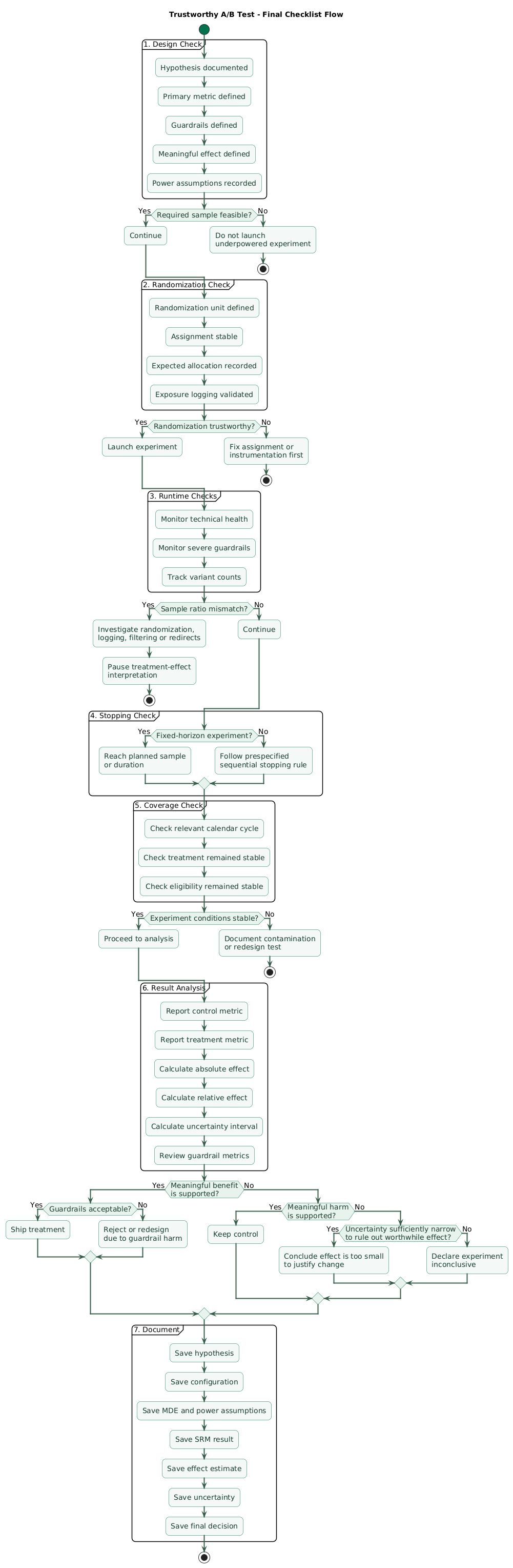
Do not launch when

• The required sample would take longer than the environment stays stable.
• The treatment cannot be randomized credibly.
• The primary outcome is too rare to measure.
• The implementation is still changing every few days.
• Telemetry is unreliable.
• The change is mandatory for legal, security, or compatibility reasons.
• You have not defined what result would change the decision.

Alternatives can include

• User research.
• Usability testing.
• Prototype testing.
• Observational analysis with explicit limitations.
• Pre/post monitoring for mandatory changes.
• Qualitative feedback.
• Combining evidence from several independent signals.

These methods do not magically provide the causal guarantees of a clean randomized experiment, but an honest weaker method can be better than a randomized experiment that has no realistic chance of answering its question.

12. Copy/paste small-traffic A/B checklist

A/B testing with small traffic checklist

Decision
- State the product decision being tested.
- Define the eligible population.
- Define the control experience.
- Define the treatment experience.
- State the expected direction of change.
- Document what result would cause treatment to ship.
- Document what result would cause treatment to be rejected.
- Allow "inconclusive" as a valid outcome.

Primary metric
- Choose one primary decision metric.
- Confirm the metric is affected by the treatment.
- Confirm the metric can be measured reliably.
- Confirm the metric has enough events for the available traffic.
- Document whether it is per user, session, account, or event.
- Avoid changing the primary metric after seeing results.

Guardrails
- Choose a small set of critical guardrail metrics.
- Include reliability or error guardrails where appropriate.
- Include customer-harm guardrails where appropriate.
- Define severe-regression stopping conditions before launch.
- Keep diagnostic metrics separate from primary decision metrics.

Minimum detectable effect
- Record the baseline metric value.
- Define the smallest effect worth acting on.
- Record the effect in absolute units.
- Record the effect as relative lift when useful.
- Do not choose the MDE only to make sample size convenient.
- Confirm smaller effects would genuinely not change the decision.

Power planning
- Choose the significance level before launch.
- Choose desired statistical power before launch.
- Calculate required observations per variant.
- Use the expected allocation ratio.
- Use eligible traffic rather than total site traffic.
- Recalculate if the baseline rate changes materially.
- Record all power assumptions.

Duration
- Convert required sample into expected calendar duration.
- Account for traffic variability.
- Cover relevant weekday/weekend cycles.
- Cover billing or purchasing cycles where relevant.
- Avoid running so long that product conditions change fundamentally.
- Do not stop simply because the sample arrives unusually quickly.

Randomization
- Define the randomization unit.
- Use user-level assignment when users return across sessions where appropriate.
- Use account or organization assignment when treatment spills over between users.
- Keep assignment stable.
- Prevent users from switching variants unexpectedly.
- Confirm randomization occurs before treatment-dependent behavior.
- Avoid post-treatment eligibility rules that bias variants.

Traffic allocation
- Prefer an efficient allocation when treatment risk allows.
- Use cautious ramp-up for potentially harmful changes.
- Avoid unnecessary experiment variants.
- Track configured allocation over time.
- Record traffic ramps and configuration changes.

Instrumentation
- Validate exposure logging.
- Validate metric logging.
- Confirm control and treatment use equivalent telemetry.
- Check for duplicate events.
- Check missing events.
- Check delayed events.
- Check variant-specific redirects.
- Check identity stitching.
- Run an A/A or similar sanity test when appropriate.

Sample ratio mismatch
- Record expected variant proportions.
- Compare observed variant counts with expected counts.
- Use an appropriate SRM statistical check.
- Investigate statistically surprising allocation differences.
- Check assignment logic.
- Check filtering.
- Check telemetry loss.
- Check bot filtering.
- Check redirects.
- Do not trust treatment effects until serious SRM issues are resolved.

Multiple metrics
- Predefine the primary metric.
- Predefine guardrails.
- Label exploratory metrics as exploratory.
- Avoid declaring success because one of many metrics happened to be significant.
- Account for multiple comparisons when the analysis requires it.

Peeking
- Decide whether the design is fixed-horizon or sequential before launch.
- For fixed-horizon tests, define the planned analysis point.
- Do not stop solely because an ordinary p-value first crosses 0.05.
- Monitor severe product regressions separately from success decisions.
- Use a statistical procedure designed for sequential monitoring when continuous stopping decisions are required.

Variance reduction
- Inspect whether the primary metric is unnecessarily noisy.
- Consider more sensitive metric definitions.
- Focus analysis on users who could actually experience treatment when the design supports triggered analysis.
- Consider pre-experiment covariates correlated with the outcome.
- Consider CUPED-style variance reduction where appropriate.
- Ensure covariates are measured before treatment.
- Avoid post-treatment variables in variance adjustment.
- Validate that variance reduction is implemented consistently.

Analysis
- Verify SRM before treatment-effect interpretation.
- Report control sample size.
- Report treatment sample size.
- Report raw event counts.
- Report control metric value.
- Report treatment metric value.
- Report absolute effect.
- Report relative effect where meaningful.
- Report uncertainty intervals.
- Report the prespecified statistical test.
- Report guardrail results.
- Report experiment duration.

Interpretation
- Do not equate p greater than alpha with proof of no effect.
- Do not equate statistical significance with practical importance.
- Compare the estimated effect with the smallest worthwhile effect.
- Consider the full uncertainty interval.
- Check whether meaningful harm remains plausible.
- Check whether meaningful benefit remains plausible.
- Treat wide uncertainty as an inconclusive result.

Segment analysis
- Avoid slicing tiny experiments into dozens of subgroups.
- Predefine critical segment hypotheses.
- Treat unexpected subgroup patterns as exploratory.
- Remember that subgroup sample sizes are even smaller.
- Replicate important subgroup findings when possible.

Experiment changes
- Avoid modifying treatment while the test is running.
- Avoid changing eligibility after observing results.
- Avoid changing the primary metric after observing results.
- Avoid changing the planned horizon only because results are unfavorable.
- Restart or clearly redesign the analysis when fundamental experiment logic changes.

Final decision
- Did randomization pass sanity checks?
- Did the experiment pass SRM checks?
- Was the planned sample or sequential stopping rule respected?
- Was relevant calendar coverage achieved?
- Is the treatment effect practically meaningful?
- Is uncertainty narrow enough for the decision?
- Did guardrails remain acceptable?
- Is the result robust enough to act on?

When not to test
- Estimate whether required sample is realistically obtainable.
- Do not launch an experiment that would take longer than the decision remains relevant.
- Do not test when randomization is impossible or unethical.
- Do not test a metric that is too rare to provide useful information.
- Do not rely on an A/B test when telemetry is unreliable.
- Consider alternative evidence for mandatory or extremely low-volume changes.

Documentation
- Save the hypothesis.
- Save the experiment configuration.
- Save the randomization unit.
- Save sample-size assumptions.
- Save the MDE.
- Save the primary metric.
- Save guardrails.
- Save stopping rules.
- Save traffic ramps.
- Save SRM results.
- Save final effect estimates and uncertainty.
- Save the decision and rationale.

13. FAQ

Can I run an A/B test with very little traffic?

Yes, when the effect worth detecting is large enough relative to the available observations and metric variability. Calculate feasibility before launch. If the required sample would take months longer than the decision remains relevant, redesign the test rather than accepting an underpowered experiment.

What is minimum detectable effect?

The MDE is the effect size the experiment is designed to detect with the selected significance level and power. A useful MDE represents the smallest difference that would materially change the product decision.

Should I stop when p becomes smaller than 0.05?

Not when using an ordinary fixed-horizon test. Repeatedly checking a conventional p-value and stopping whenever significance first appears changes the statistical procedure. Use the predefined horizon or a method designed explicitly for sequential monitoring.

What is sample ratio mismatch?

SRM occurs when observed variant counts differ unexpectedly from the configured allocation. It can indicate problems in assignment, telemetry, filtering, redirects, eligibility, or data processing. Investigate it before trusting treatment effects.

How can I increase power with limited traffic?

Focus on users actually eligible for treatment, choose a sensitive primary metric, reduce avoidable variance, avoid unnecessary variants, improve instrumentation, and consider pre-experiment covariates or CUPED-style variance reduction when appropriate.

Does a non-significant result mean the variants are the same?

No. A non-significant result may simply reflect insufficient precision. Examine the estimated effect and its uncertainty interval to determine whether meaningful improvement or harm remains plausible.

Key terms (quick glossary)

A/B test

A randomized controlled experiment comparing two product experiences, commonly a control and a treatment.

Randomization unit

The entity independently assigned to an experiment variant, such as a user, account, organization, device, or session.

Minimum detectable effect (MDE)

The smallest treatment effect an experiment is designed to detect with specified statistical power and significance level.

Statistical power

The probability that a test correctly rejects its null hypothesis when the specified alternative effect is truly present.

Significance level

A prespecified probability threshold controlling the Type I error rate under the assumptions of the statistical testing procedure.

Type I error

Rejecting the null hypothesis when it is actually true.

Type II error

Failing to reject the null hypothesis when the specified alternative is true.

Guardrail metric

A metric monitored to ensure that an experiment does not cause unacceptable harm while improving its primary outcome.

Sample ratio mismatch (SRM)

A statistically unexpected difference between the configured experiment allocation and the observed counts assigned or measured in each variant.

Optional stopping

A practice in which the time an experiment ends depends on results observed while data is accumulating.

Sequential testing

A statistical design that explicitly allows repeated analyses or stopping decisions while preserving defined error properties.

CUPED

A variance-reduction approach that uses relevant pre-experiment information to explain baseline variability in experiment outcomes.

Triggered analysis

Analysis focused on randomization units that reached a prespecified eligibility or exposure condition relevant to the treatment.