AI inference looks cheap in prototypes and expensive in production for one reason: production traffic forces you to pay for long prompts, long outputs, low utilization, retries, and multi-call workflows. If you want predictable unit economics, you need a cost model, the right metrics, and a rollout plan that reduces spend without breaking latency SLAs or quality.
A proven optimization order
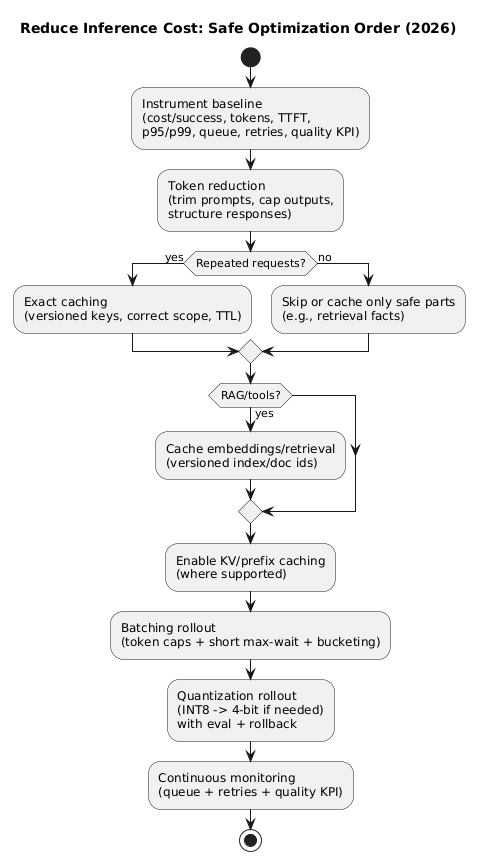
Most teams see the best results by optimizing in this order: measure → reduce tokens → cache → batch → quantize. Each step compounds the next.
1. The real cost drivers (why spend spikes)
Inference costs typically rise because multiple small factors compound:
- Context creep: system prompts and chat history expand over time.
- Output creep: outputs get longer unless you enforce limits and formats.
- Utilization gaps: GPUs sit partially idle when requests are served one-by-one.
- Reliability overhead: retries, timeouts, and duplicate requests multiply spend.
- Multi-call pipelines: RAG + tools + safety checks turn one action into 2–5 calls.
- Tail latency: outliers trigger client retries and amplify traffic.
A common hidden multiplier
A single “answer this question” can become: embeddings → retrieval → generation → re-rank → regeneration on tool error → safety re-check. If you do not track “calls per user action,” you will underestimate cost by multiples.
2. A useful cost model: prefill vs decode (and why it matters)
You do not need a perfect model, but you do need a useful one. A practical decomposition is:
- Prefill cost: processing the input context (system + user + retrieved text).
- Decode cost: generating output tokens (token-by-token).
- Memory pressure: long contexts inflate KV cache and increase OOM risk.
- Utilization: how well you keep hardware busy (batching/scheduling/concurrency).
Decision shortcut
If input tokens are high, prioritize token reduction and KV/prefix caching. If traffic volume is high and utilization is low, prioritize batching. If memory is the constraint, prioritize quantization and context policies.
3. What to measure: dashboards that prevent bad optimizations
Optimizations fail when teams watch only one number (e.g., average latency). Track these per endpoint, per model route, and ideally per tenant (if multi-tenant).
3.1 Cost and usage
- Cost per successful request (separate failed calls and retries).
- Input tokens and output tokens (p50/p95).
- Calls per user action (especially for RAG/tool workflows).
- Tokens per outcome (best metric when you can define “outcome”).
3.2 Latency, throughput, saturation
- Latency percentiles: p50/p95/p99 (tail latency drives retries).
- Queue time: critical when batching is enabled.
- TTFT: time-to-first-token (user perceived speed).
- Tokens/sec: decode throughput under steady load.
- GPU utilization: compute and memory, plus idle vs active time.
3.3 Reliability and quality
- Timeout/OOM rates and provider error rate.
- Retry rate and duplicate request rate (cost amplifiers).
- Quality KPI: task success, acceptance, escalation, CSAT, or completion rate.
4. Token reduction: the highest-leverage first step
Before caching, batching, or quantization, reduce the number of tokens you send and generate. This is the one lever that typically improves cost and latency together.
4.1 Prompt trimming that does not break behavior
- Version your system prompt and remove duplicated policy text.
- Prefer concise rules (bullets) over long paragraphs.
- Move examples out of the hot path unless they materially lift quality.
- Summarize chat history and keep only turns that affect the next action.
4.2 Output shaping and caps
- Set endpoint-specific max output tokens (treat as a product contract).
- Use structured outputs (JSON schema) for workflows to reduce verbosity and rework.
- Stop early when the required structure is complete.
5. Caching deep dive: exact, semantic, retrieval, KV/prefix
Caching reduces cost by not doing work. But you need the right caching layer, correct scoping, and safe invalidation—or you will create correctness and privacy incidents.
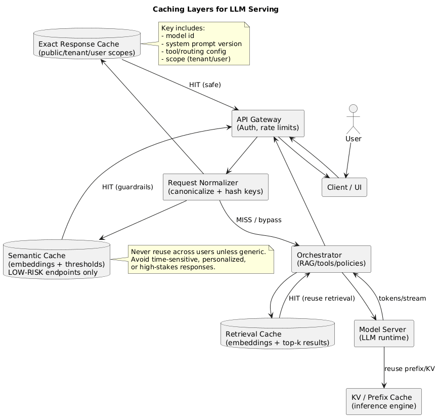
5.1 Exact response/prompt caching (best first move)
Exact caching returns a stored response for requests that match (after normalization). It is ideal for templates, repeated questions, internal tooling prompts, and stable FAQs.
- Key design: hash normalized prompt + model ID + system prompt version + routing/tool config.
- Scope: public vs tenant vs user cache (never mix scopes).
- TTL: short TTL for time-sensitive outputs; longer TTL for stable outputs.
- Safety: avoid caching personalized outputs unless cache is user-scoped.
5.2 Retrieval and embedding caching (RAG stability win)
If you use RAG, caching embeddings and top-k retrieval results can reduce overhead and stabilize latency. Keep invalidation tied to index/document versions so you do not serve stale facts indefinitely.
5.3 Semantic caching (higher hit rate, higher risk)
Semantic caching reuses a previous answer when a new query is similar enough (typically via embeddings). It can be valuable for generic, low-risk endpoints, but it fails when two queries are “similar” with one critical difference.
- Use strict thresholds and tune on real traffic.
- Avoid high-stakes domains and time-sensitive/personalized outputs.
- Prefer “reuse facts, regenerate answer” when similarity is borderline.
5.4 KV cache and prefix caching (compute savings for long contexts)
KV caching avoids recomputing attention states for the same prefix during generation. It helps most when: prompts are long, sessions are multi-turn, or streaming decode dominates.
- Watch memory: KV cache can dominate memory for long contexts.
- Measure eviction: high eviction rate reduces benefits and increases variance.
- Version shared prefixes: prefix caching benefits from stable, versioned system prompts.
6. Batching deep dive: dynamic, continuous, bucketing, guardrails
Batching reduces cost by improving utilization: more tokens processed per unit of GPU time. The trade-off is queue time and tail latency, so batching must be engineered with guardrails.
6.1 Dynamic vs continuous batching
- Dynamic batching: batch requests arriving within a short time window.
- Continuous batching: keep the GPU busy by continuously merging and advancing requests.
6.2 The three batching guardrails that prevent regressions
- Token-based caps: cap by total tokens per batch, not only by request count.
- Short max-wait: keep queue time bounded to protect p95/p99 latency.
- Length bucketing: group similar prompt lengths to avoid padding waste and “long-request poisoning.”
Batching can increase total spend
If batching increases tail latency enough to trigger retries, total compute rises and costs go up. Always monitor queue time and retry/duplicate-request rates during rollouts.
6.3 Streaming-specific considerations
- TTFT is sensitive to queue time and prefill scheduling.
- Tokens/sec is sensitive to decode scheduling, KV cache efficiency, and quantization kernels.
- Fairness: ensure one long stream cannot starve shorter interactive requests.
7. Quantization deep dive: INT8 vs 4-bit, calibration, rollout
Quantization reduces cost primarily via lower memory and potentially higher throughput. The real-world outcome depends on hardware and kernel support, so you must benchmark on your workload.
7.1 What typically gets quantized
- Weights: the most common, often “weight-only” quantization.
- Activations: can bring speedups but requires careful kernel support.
- KV cache: can reduce memory pressure for long contexts (when supported).
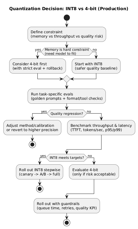
7.2 Choosing INT8 vs 4-bit
- INT8: safer baseline with strong memory savings and often minimal regressions.
- 4-bit: consider when memory is the constraint (fit larger models) or when throughput gains justify stricter evaluation.
7.3 PTQ vs QAT (what to do first)
- PTQ: fastest path; quantify after training. Start here for most teams.
- QAT: can preserve quality better but requires training and careful experiments.
7.4 Validation: what to test (non-negotiable)
- Task evals: representative prompts, structured-output correctness, and tool-call reliability.
- Regression suite: “golden prompts” with strict formatting checks.
- Safety behavior: ensure refusals and policy constraints do not degrade.
- Quality KPI: monitor acceptance/escalation/CSAT during rollout.
8. A safe rollout playbook (order that works)
- Freeze a baseline: tokens, p95/p99 latency, TTFT, tokens/sec, retries, quality KPI.
- Reduce tokens: trim prompts, cap outputs, structure responses.
- Add exact caching: versioned keys, correct scope, TTL; then retrieval caching if RAG.
- Enable batching: token caps, short max-wait, bucketing; watch queue time and retries.
- Quantize stepwise: INT8 → 4-bit if needed; benchmark; keep rollback routing.
- Lock in governance: config versioning, change logs, incident playbooks.
Why order matters
Shorter prompts reduce KV memory, which allows larger safe batches, which improves throughput. That makes quantization benefits easier to realize. Done out of order, you often trade one problem for another.
9. Reference architectures that reduce cost
9.1 Split interactive and background inference
Separate latency-sensitive endpoints from background jobs (offline summaries, enrichment). This lets you use different batching windows, token caps, and autoscaling policies.
9.2 Multi-model routing (small model first)
Route easy requests to smaller models and hard requests to larger models. This reduces average cost while preserving quality where it matters. Routing works best when you instrument outcomes and define clear thresholds.
9.3 CPU for retrieval and orchestration, GPU for generation
Keep “non-GPU work” off the GPU: routing, retrieval, lightweight validation, and formatting checks can often run on CPU. This improves effective GPU utilization and reduces queue pressure.
10. Practical checklist (copy/paste)
- Instrument cost per successful request, tokens (p50/p95), TTFT, p95/p99 latency, queue time, retries, OOM/timeout.
- Reduce tokens: trim prompts, summarize history, cap outputs, prefer structured responses.
- Exact cache first: versioned keys, correct scoping, safe TTLs, secure retention.
- Cache retrieval (embeddings/top-k) to stabilize RAG and reduce repeated work.
- KV/prefix caching where supported; monitor memory pressure and eviction.
- Batching: token caps + short max-wait + bucketing; watch queue time and retry rate.
- Quantize stepwise: INT8 → 4-bit (if needed) with task evals and rollback routing.
- Guardrails: quality KPI must be monitored continuously; treat regressions as incidents.
11. Frequently Asked Questions
What is the quickest way to reduce AI inference costs?
Start with measurement (cost per successful request and token distributions), then reduce tokens by trimming prompts and capping outputs. Next, implement exact caching for repeated requests—this often delivers immediate savings without changing model behavior.
Which caching should I implement first: exact, semantic, or KV cache?
Implement exact response/prompt caching first for safe, repeated requests. Add retrieval/embedding caching if you use RAG. Use KV/prefix caching when prompts are long or sessions are multi-turn. Consider semantic caching only for low-risk endpoints with strict similarity thresholds and correct scoping.
Does batching always reduce inference cost per request?
Batching usually improves throughput and utilization, lowering cost per token. However, it can increase tail latency if the system waits too long to form batches, or if long requests dominate batch composition. Use token-based caps, short max-wait windows, and monitor queue time and retries.
How do I choose between INT8 and 4-bit quantization?
Start with INT8 when you want safer quality with solid memory savings. Consider 4-bit when memory is the hard constraint (fitting a model on available GPUs) or when the throughput gain is worth stricter evaluation. Always validate on task-specific tests and keep a rollback route.
Which metrics matter most during inference cost optimization rollouts?
Track cost per successful request, input/output tokens, tokens/sec, TTFT, p50/p95/p99 latency, queue time, cache hit rates, OOM/timeout rates, retry/duplicate request rates, and a clear quality KPI (task success, CSAT, escalation). Optimize with guardrails so one metric doesn’t silently worsen another.
Key terms (quick glossary)
- Prefill
- The phase where the model processes the input context (system + user + retrieved text) before generating output tokens.
- Decode
- The token-by-token generation phase. Costs scale with output length and concurrency.
- TTFT
- Time to first token. Strongly impacted by queue time and prefill scheduling.
- Exact cache
- Returning stored outputs for requests that match exactly (after normalization and versioning).
- Semantic cache
- Reusing outputs for “similar enough” requests (typically via embeddings). Requires strict guardrails and safe scoping.
- KV cache
- Stored attention states that reduce recomputation for repeated prefixes and long contexts.
- Dynamic batching
- Automatically forming batches within a short time window to improve utilization.
- Continuous batching
- Scheduling that continuously merges and advances requests to keep the GPU busy under streaming and mixed arrivals.
- Quantization
- Using lower-precision formats (INT8/4-bit) for weights/activations/KV cache to reduce memory and potentially increase throughput.
- Cost per successful request
- Unit cost excluding failed calls; track failures/retries separately to avoid hiding regressions.
Worth reading
Recommended guides from the category.